Notebook(Final)

Final Version

Loading some Packages for Better Presentation of Results

library(gt)
library(ggplot2)
library(tidyr)
library(dplyr)

Attache Paket: 'dplyr'

Die folgenden Objekte sind maskiert von 'package:stats':

    filter, lag

Die folgenden Objekte sind maskiert von 'package:base':

    intersect, setdiff, setequal, union

set.seed(1)

Definitions

Initial Population

Norm Population

Initial Populations In line with the paper, a population is generated where the money is normally distributed with a mean of 100.

To save computation time, the number of agents is reduced from 5000 to 1500. Additionally, the population is sorted and assigned an ID to track them. Agents with small IDs receive the least money, while agents with large IDs have a lot of money.

nA = 1500         # number of Agents
ID = seq_len(nA)  # ID of the Agents
M0pop = 100       # Mean amount of Money in the Start-Population

PopNorm <- data.frame( ID = ID,
                       Money= sort(rnorm(nA, mean = M0pop, sd = 0.2 * M0pop))
                      )

Equal Population

Also in line with the paper, a second population is generated where all agents start with the same amount of money.

PopEqual <- data.frame( ID = ID,
                       Money = rep(M0pop, times = nA)
                      )

Functions

Gini-Faktor

To describe the distribution of money in the population, a function is defined to calculate the Gini coefficient.

Needs

1. Vector with Money distribution

Output

1. Gini-Factor

gini <- function(VM) {
  VM <- sort(VM)
  n <- NROW(VM)
  numer <- 0
  for (i in 1:n) {
    numer <- numer + 2 * i * VM[i]
  }
  denom = n * sum(VM)
  return((numer / denom) - (n + 1) / n)
}

Timeline

The same is also implemented as a time function.

Needs

1. Matrix with Money distribution as vector per time

Output

1. Vector with Gini-Factor per time

gini_t <- function(MM) {
  n <- NCOL(MM)
  GT <- c(0)
  for (i in 1:n) {
    GT[i] <-  gini(MM[,i])
  }
  return(GT)
  }

Transaction rule

In line with the paper, a random distribution of money between two agents is defined.

Needs

1. Nothing

Output

1. Vector with a random number and 1minus this number

splitpair <- function(){
  rn <- runif(1)
  c(rn,1-rn)
}
splitpair()

[1] 0.8023495 0.1976505

Probabilities

Since it was suspected in the sketchbook that the reason for the outcome is the decreasing probability of meeting an agent with more or a lot of money, a function is defined here to calculate various probabilities:

• Probability of winning money (probwin)

• Probability of having more money than the current median in the population after the exchange (probmed)

• Probability of having more money than the mean in the population after the exchange (probmean)

Needs

1. Vector with Money distribution

Output

1. Summary (Sum) with minimum, maximum, median and mean for the given Money and the mention probabilities

2. Distribution (Dist) for the same values

calc_p_s <- function(VM) {
  Dist <- data.frame(Money = VM,
                     probwin = 0,
                     probmed = 0,
                     probmean = 0
                     )
  Sum <- data.frame(Money = c(min(Dist$Money),
                              max(Dist$Money),
                              median(Dist$Money),
                              mean(Dist$Money)
                              ),
                    probwin = 0,
                    probmed = 0,
                    probmean = 0
                    )
  rownames(Sum) <- c("min", "max", "med", "mean")
  M_Med <- Sum["med", "Money"]
  M_Mean <- Sum["mean", "Money"]
  for(i in 1:nrow(Dist)) {
    M_A <- Dist[i,"Money"]
    M_oA <- Dist[c(-i),"Money"]
    pwin <- M_oA*0
    pmed <- M_oA*0
    pmean <- M_oA*0
    for(ii in 1:NROW(M_oA)) {
      Pot <- max(M_A + M_oA[ii], 10e-8)
      pwin[ii] <- 1-min(1, M_A/Pot)
      pmed[ii] <- 1-min(1, M_Med/Pot)
      pmean[ii] <- 1-min(1, M_Mean/Pot)
    }
    Dist[i,"probwin"] <- mean(pwin)
    Dist[i,"probmed"] <- mean(pmed)
    Dist[i,"probmean"] <- mean(pmean)
  }
  for (i in c("probwin","probmed","probmean")) {
    Sum[[i]] = c(min(Dist[[i]]),
                    max(Dist[[i]]),
                    median(Dist[[i]]),
                    mean(Dist[[i]])
    )
  }

  Output <- list(Sum = Sum, Dist = Dist)
  return(Output)
}

The same Function with matrix calculations, what is much faster!

calc_p <- function(VM, Detailed=FALSE) {
  n <- length(VM)
  ID <- seq(1:n)
  MM <- matrix(rep(VM,times=n),n,n)
  S <- (VM + t(MM))
  S[S==0] <- 10e-6
  pwin <- (1 - t(MM)/S)
  diag(pwin) <- 0
  pmed <- 1-(median(VM)/S)
  pmed[pmed<0] <- 0
  diag(pmed) <- 0
  pmean <- 1-(mean(VM)/S)
  pmean[pmean<0] <- 0
  diag(pmean) <- 0

  Dist <- data.frame(Money = VM,
                     probwin = colSums(pwin)/(n-1),
                     probmed = colSums(pmed)/(n-1),
                     probmean = colSums(pmean)/(n-1)
  )

  Sum <- data.frame(Money = c(min(Dist$Money),
                              max(Dist$Money),
                              median(Dist$Money),
                              mean(Dist$Money)),
                    probwin = c(min(Dist$probwin),
                                max(Dist$probwin),
                                median(Dist$probwin),
                                mean(Dist$probwin)),
                    probmed = c(min(Dist$probmed),
                                max(Dist$probmed),
                                median(Dist$probmed),
                                mean(Dist$probmed)),
                    probmean = c(min(Dist$probmean),
                                 max(Dist$probmean),
                                 median(Dist$probmean),
                                 mean(Dist$probmean))
  )

  rownames(Sum) <- c("min", "max", "med", "mean")
  Output <- list(Sum = Sum, Dist = Dist)
  if (Detailed) {
    D <- data.frame(t(pmed))
    diag(D) <- colSums(pmed)/(n-1)
    D <- round(D, digits=2)
    D <- format(D, digits=2)
    VMm <- round(median(VM), digits=1)
    VMm <- format(VMm, digits=4)
    VM <- round(VM, digits=1)
    VM <- format(VM, digits=4)
    D <- rbind(VM, D)
    D <- cbind(c("Money",ID),c(VMm,VM), D)
    colnames(D) <- c("ID","Money",ID)
    D <- gt(D)
    D <- tab_spanner(D, label = "Probabilities", columns = 3:(n+2))
    for (i in 1:(n + 1)) {
      if (i==1) {
        D <- tab_style(D,
                       style = list(cell_text(style = "italic")),
                       locations = cells_body(i+1,))
        D <- tab_style(D,
                       style = list(cell_text(style = "italic")),
                       locations = cells_body(,i))
        }
      D <- tab_style(D,
                     style = list(cell_text(weight = "bold")),
                     locations = cells_body(i+1, i))
    }
    D <- tab_source_note(
      D,
      source_note = "Italic/bold = Median of Money, Bold = Mean in the Population"
    )
    Output$SumD <- D
  }
  return(Output)
}

Timeline

The same is also implemented as a time function.

Needs

1. Matrix with Money distribution as vector per time ( as reported from ecosim$timeline)

Output

1. Matrix probability-values per time in colones (long form)

calc_p_t <- function(MM) {
  pnt <- calc_p(MM[,1])
  tx <- as.numeric(gsub("n", "",colnames(MM)[1]))
  pnts <- data.frame(Time = rep(tx, times = 4),
                     Res = colnames(pnt$Sum),
                     t(pnt$Sum)
                     )
  for(i in 2:ncol(MM)) {
    pnt <- calc_p(MM[,i])
    tx <- as.numeric(gsub("n", "",colnames(MM)[i]))
    pnti <- data.frame(Time = rep(tx, times = 4),
                       Res = colnames(pnt$Sum),
                       t(pnt$Sum)
                       )
    pnts <- rbind(pnts,pnti)
  }
  rownames(pnts) <- NULL
  return(pnts)
}

Economic Simulation

Finally, a simulation is created that simulates a certain number of money exchanges.

Needs

1. Number of exchanges

2. Startdistribition of Money

3. Steps for the timeline (optional)

Output

1. Summary (Sum) with ID, number of exchanges, Money at beginning and Money at the End

2. Matrix with Money distribution(Timeline) for given time steps as vectors (if steps > 0)

ecosim <- function( n, VM, TL = 0 ) {
  df <- data.frame(ID=seq(1,NROW(VM)),
                   nE=0,
                   MT_S=VM,
                   MT_E=VM
                   )
  if (TL > 0) {
    M_TL <- data.frame(n0 = df$MT_S)
  }
  for(i in 1:n) {
    rdf <- sample(df$ID, size=2)
    rds <- splitpair()
    df[rdf,"nE"] <- df[rdf,"nE"] + 1
    df[rdf,"MT_E"] <- sum( df[rdf,"MT_E"]) * rds
    if ( TL > 0 ) {
      if ( i %% TL == 0) {
        M_TL [[paste0("n",i)]]<- df$MT_E
      }
    }
  }
  Output <- list("Sum" = df)
  if ( TL > 0 ) {
    rownames(M_TL) <- df$ID
    Output$Timeline <- M_TL
  }
  return(Output)
}

Plot functions

Histogram

Needs

1. Summary of a economic Simulation

figHist <- function(Sim_Sum) {
  Fig <- pivot_longer(data.frame(Sim_Sum),
                      cols = starts_with("MT"),
                      names_to = "Distribution",
                      values_to = "Money"
                      )
  Fig$Distribution <-recode(Fig$Distribution,
                            "MT_S" = "at Begining",
                            "MT_E" = "at the End"
                            )
  Figp <- ggplot(Fig, aes(x = Money, fill = Distribution)) +
    geom_histogram(position = "identity", alpha = 0.5, bins = 50) +
    ylab("Frequency") +
    scale_fill_manual(name = NULL, values = c(4,3)) +
    scale_color_manual(name = NULL, values = c(4, 3)) +
    theme_minimal() +
    theme(legend.position = "top")
  return(Figp)
}

Probabilities in the Population

Needs

1. Probability distribution from calc_p

2. Title for the figure

3. Maximum for the x axis (Money)

figProb <- function(Prob, Title, xmax) {
  Figd <- pivot_longer(data.frame(Prob$Dist),
                       cols = starts_with("p"),
                       names_to = "Outcome",
                       values_to = "Probability"
                       )
  Figs <- Prob$Sum

  Figp <- ggplot(data = Figd,
                 aes(x = Money,
                     y = Probability,
                     color = Outcome
                     )
                 ) +
    geom_point( alpha = 0.5, size = 1.5) +
    scale_color_manual(name = "Probability to",
                       values = c(2, 3, 4),
                       labels = c("gain more than the Mean",
                                  "gain more than the Median",
                                  "gain")
                       ) +
    ylim(0, 1) +
    xlim(0, xmax) +

    geom_vline(xintercept = Figs["med","Money"],
               linetype = "solid", color = 1) +
    annotate("text",
             x = Figs["med","Money"] * 0.95,
             y = 0,
             hjust = 1,
             vjust = 0,
             label = paste("Median\n=",
                           round(Figs["med","Money"], 0)),
             color = 1) +

    geom_vline(xintercept = Figs["mean","Money"],
               linetype = "dashed", color = 1) +
    annotate("text",
             x = Figs["mean","Money"] * 1.05,
             y = 0,
             hjust = 0,
             vjust = 0,
             label = paste("Mean\n=",
                           round(Figs["mean","Money"], 0)),
             color = 1) +

    geom_hline(yintercept = Figs["mean","probmed"],
             linetype = "solid", color = 3) +
    annotate("text",
             x = xmax,
             y = Figs["mean","probmed"] * 1.05,
             hjust = 1,
             vjust = 0,
             label = paste("Mean =",
                           round(Figs["mean","probmed"], 2)),
             color = 3) +

    geom_hline(yintercept = Figs["mean","probmean"],
               linetype = "solid", color = 2) +
    annotate("text",
             x = xmax,
             y = Figs["mean","probmean"]*0.95,
             hjust = 1,
             vjust = 1,
             label = paste("Mean =",
                           round(Figs["mean","probmean"], 2)),
             color = 2) +

    labs(title = Title) +
    theme_light() +
    theme(legend.position = "top",
          legend.justification = c(0, 1))
  return(Figp)
}

Probabilities over Time

Needs

1. Probability distribution from calc_p_t

2. Title for the figure

figProb_t <- function(Prob, Title) {
  Fig <- Prob[Prob$Res!="Money",c("Time","Res","mean")]

  Figp <- ggplot(data = Fig, aes(x = Time, y = mean, color = Res)) +
    geom_line(linewidth = 1) +
    scale_color_manual(name = NULL, values = c(2, 3, 4),
                      labels = c("gain more than the Mean",
                                 "gain more than the Median",
                                 "gain")) +
    ggtitle(Title) +
    xlab("number of exchanges") +
    ylab("Mean-Probability in the Population") +
    ylim(0.30, 0.6) +
    theme_light() +
    theme(legend.position = "top",
         legend.justification = c(0, 1))
  return(Figp)
}

Simulation for…

Normal Population

Simulation for 60000 exchanges with output after every 500th exchange.

sNorm <- ecosim(60000, PopNorm$Money, TL = 250)

Presentation of the end results

At the beginning, the distribution of money in the population looks like this. After simulating 60000 money exchanges, the following distribution emerges.

Fig01 <- figHist(sNorm$Sum)
Fig01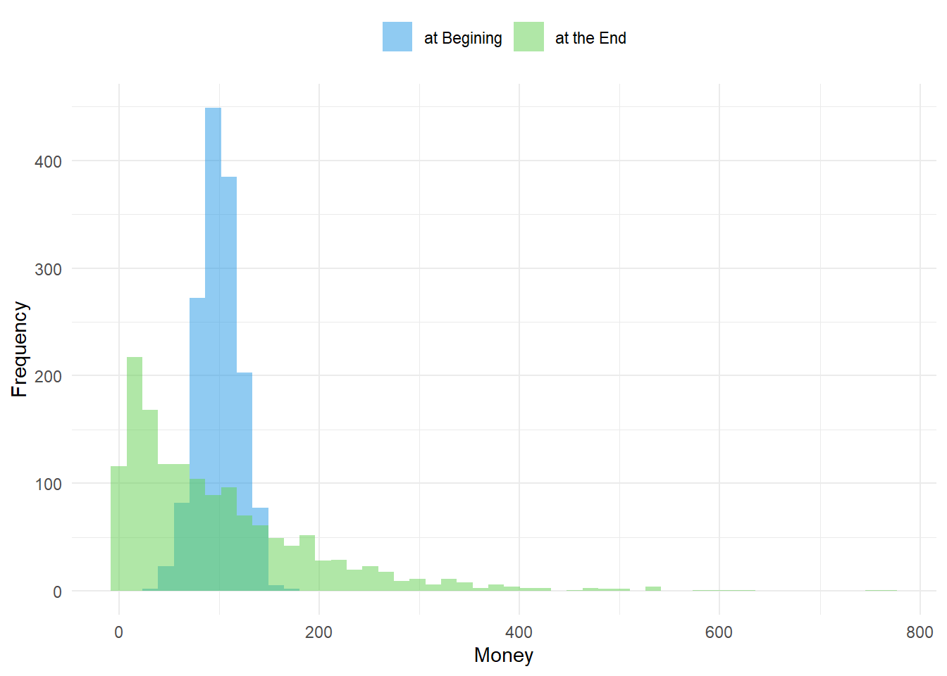

Representation of Money over time

It seems that every agent has the chance to have a lot of money in the end. This can be shown by tracking individual agents and their money. Below, nine agents are shown: three with little, three with 100, and three with the most money at the beginning.

MTime <- data.frame(ID,sNorm$Timeline)

sID <- c(1,2,3,nA/2-1,nA/2,nA/2+1,nA-2,nA-1,nA)
sMTime <- MTime[sID,]

Fig02 <- pivot_longer(data.frame(sMTime),
                      cols = !matches("ID"),
                      names_to = "Time",
                      names_prefix = "n",
                      names_transform = list(Time = as.integer),
                      values_to = "Money"
)

Fig02$ID <- sprintf("%04d", Fig02$ID)

ggplot(data = Fig02, aes(x = Time, y = Money, color = ID)) +
  geom_line() +
  ggtitle("Timeline for some Agents") +
  xlab("number of exchanges") +
  labs(color = "Agents ID") +
  scale_color_manual(values = c(2,2,2, 1,1, 1,3,3,3)) +
  theme_light() +
  theme(legend.position = "right",
        legend.justification = c(0, 1))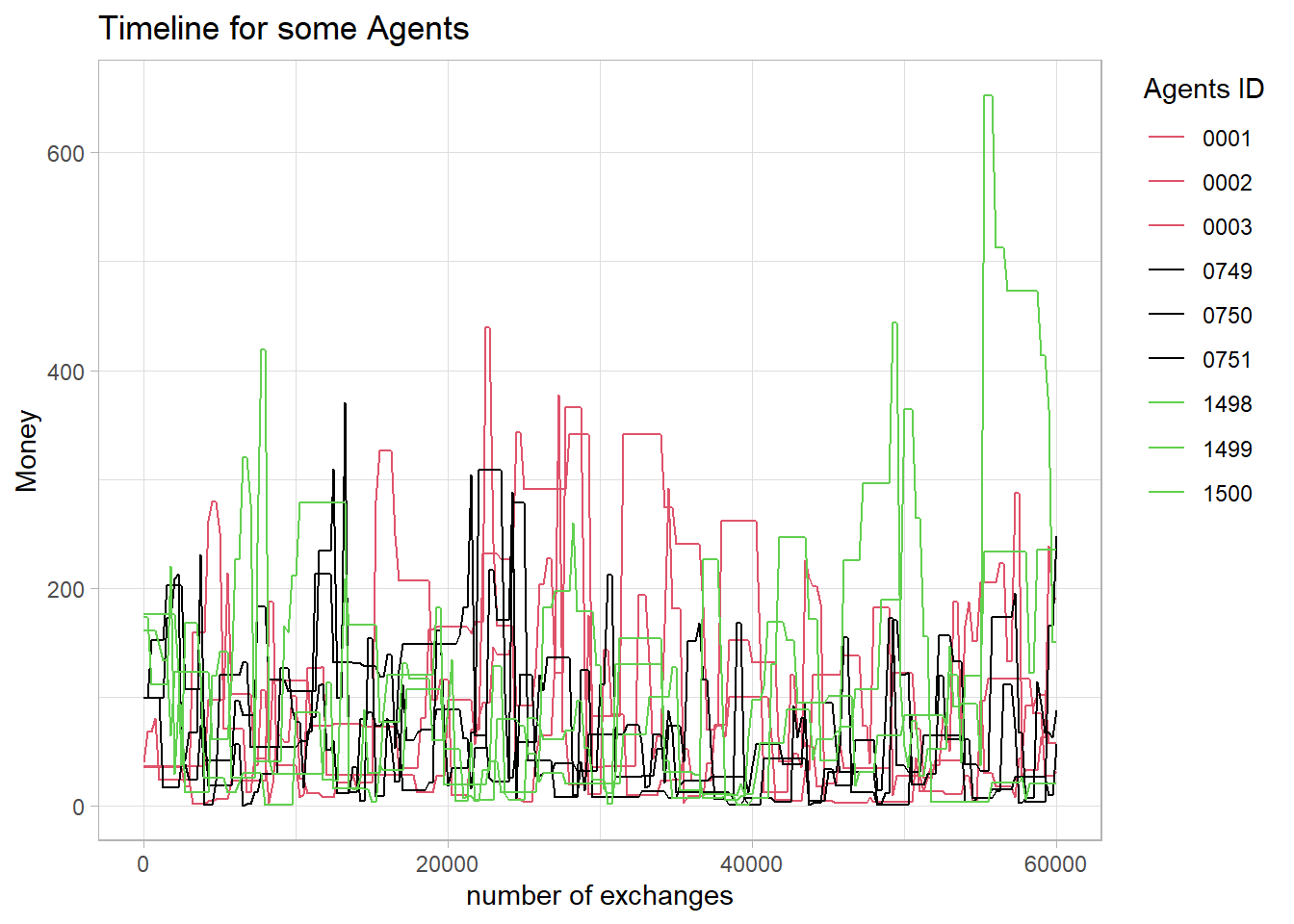

Probabilities for specific Timesteps

This can also be shown with the calculated probabilities for the next meeting for each agent.

Fig03 <- figProb(calc_p(sNorm$Timeline[,1]), 
                "Probability at Beginning", 850)
Fig04 <- figProb(calc_p(sNorm$Timeline[,3]), 
                "Probability after 500 exchanges", 850)
Fig05 <- figProb(calc_p(sNorm$Timeline[,5]), 
                "Probability after 1000 exchanges", 850)
Fig06 <- figProb(calc_p(sNorm$Timeline[,NCOL(sNorm$Timeline)]), 
                "Probability at the End", 850)

Initially, it seems to be a fairly fair trade, so agents with little money have a higher probability of winning money in the next exchange. However, they also have a lower probability of ending up above the median or the mean. At the beginning, all probabilities in the population are about 0.5 on average.

Fig03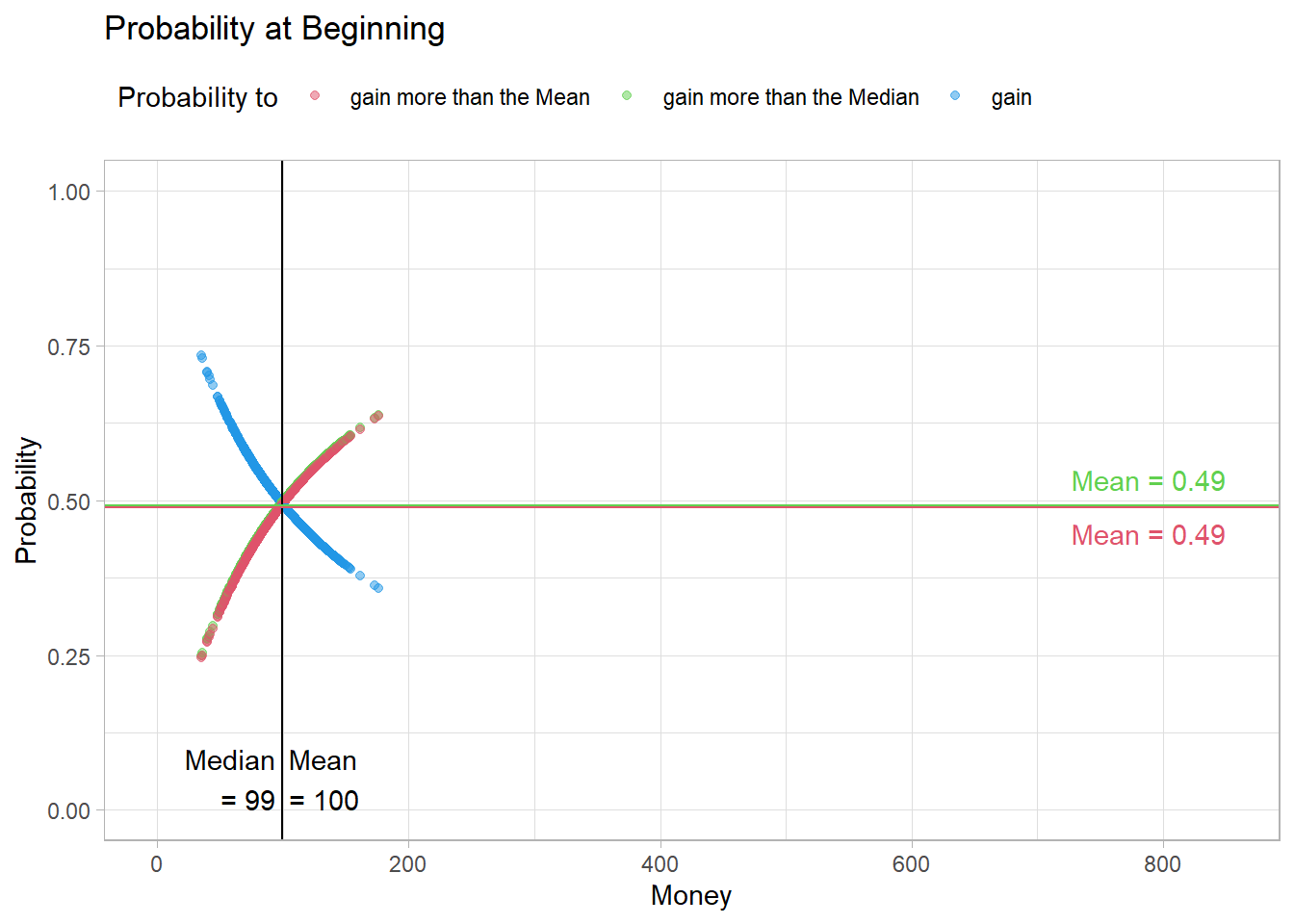

However, after a few meetings, this changes. The probability of ending up above the median or the mean decreases.

The reason for this is that with each exchange, a rich and a poor agent are created, which decreases the probability of meeting a rich agent in the future. As a result, the median amount of money decreases.

Fig04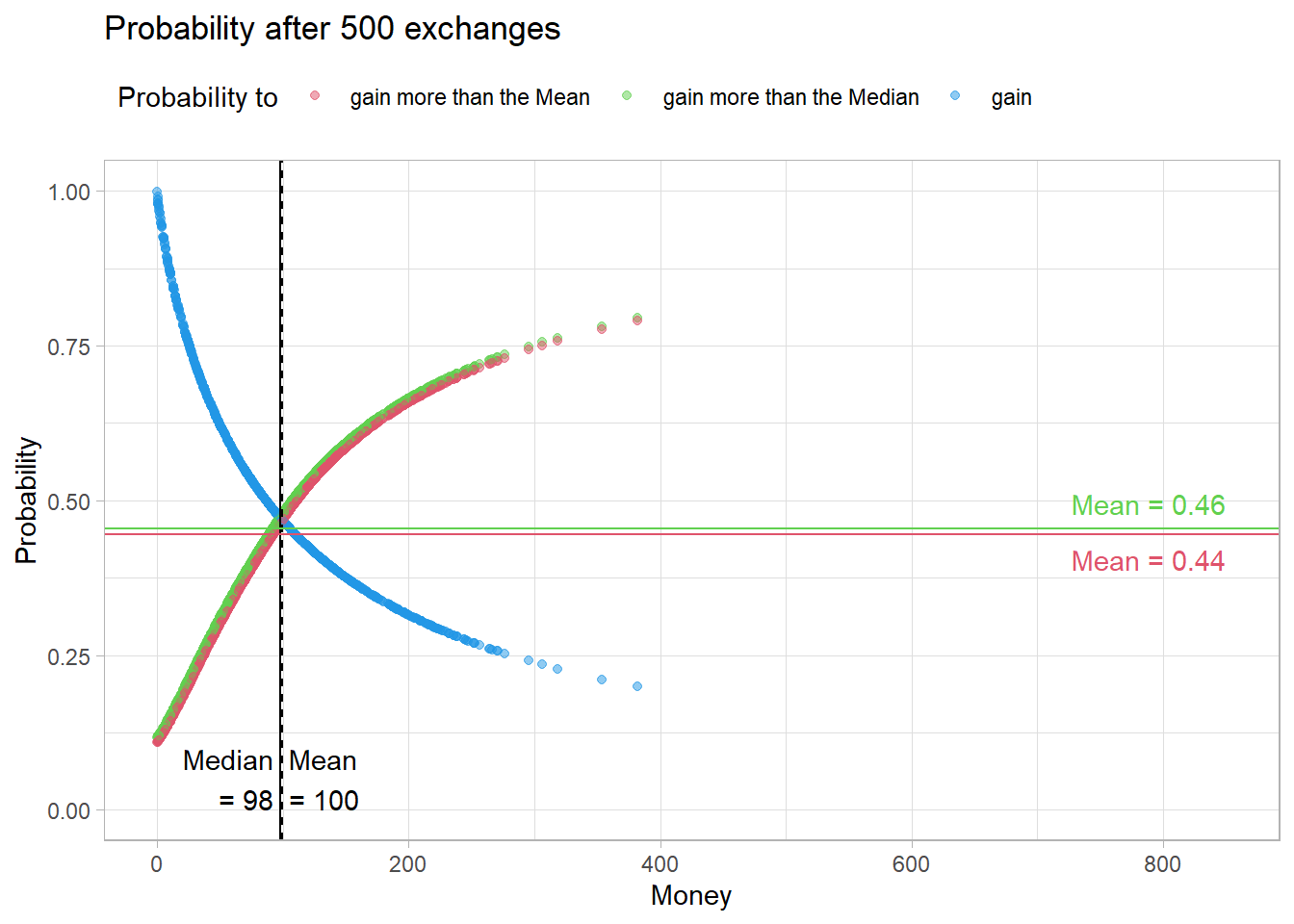

This effect intensifies over time.

Fig05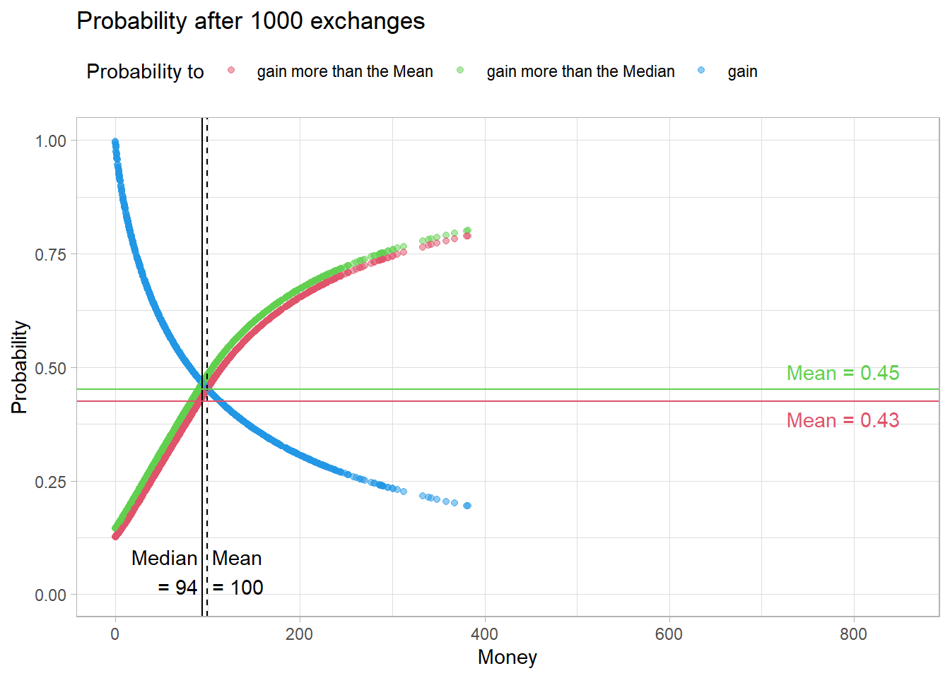

After 60000 meetings, the distribution of probabilities in the population looks like this.

Fig06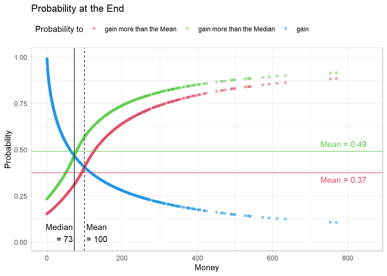

It seems that the probability of ending up above the median rises back to 0.5. However, the probability of ending up above the mean remains low.

Probabilities over Time

ProbNormt <- calc_p_t(sNorm$Timeline)

This can be seen even better when looking at the said probabilities over time.

Fig07 <-figProb_t(ProbNormt, "Probability to ... of Money - Timeline")
Fig07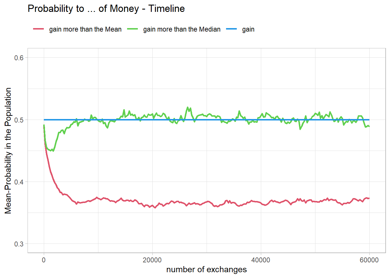

Equal Population

Simulation for 60000 exchanges with output after every 250th exchange.

eNorm <- ecosim(60000, PopEqual$Money, TL = 250)

Presentation of the end results

At first glance, it seems illogical that a population where everyone starts with the same amount of money would result in a similar final distribution of money. However, the simulation proves this.

Fig08 <- figHist(eNorm$Sum)
Fig08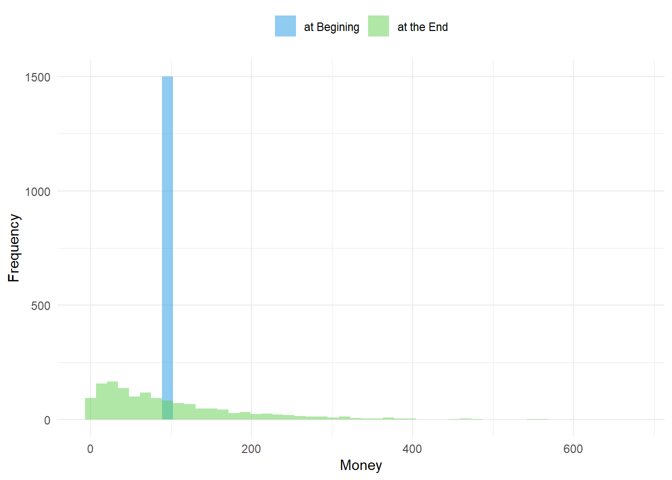

Probabilities for specific Timesteps

Fig09 <- figProb(calc_p(eNorm$Timeline[,1]), 
                "Probability at Beginning", 850)
Fig10 <- figProb(calc_p(eNorm$Timeline[,3]), 
                "Probability after 500 exchanges", 850)
Fig11 <- figProb(calc_p(eNorm$Timeline[,5]), 
                "Probability after 1000 exchanges", 850)
Fig12 <- figProb(calc_p(eNorm$Timeline[,NCOL(eNorm$Timeline)]), 
                "Probability at the End", 850)

At the beginning, all probabilities are exactly 0.5.

Fig09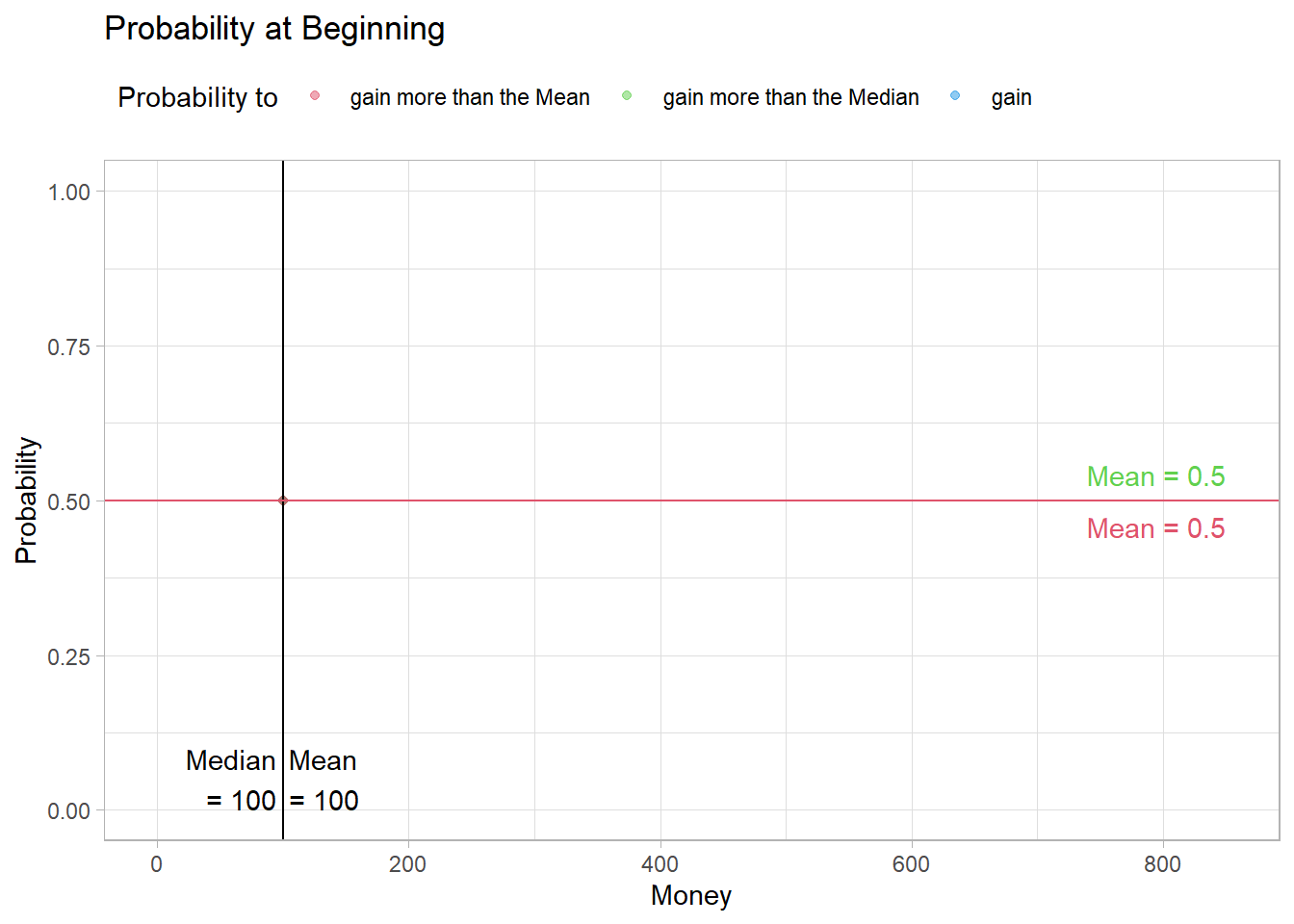

However, the same mechanism applies here. With each exchange, a rich and a poor agent are created.

Fig10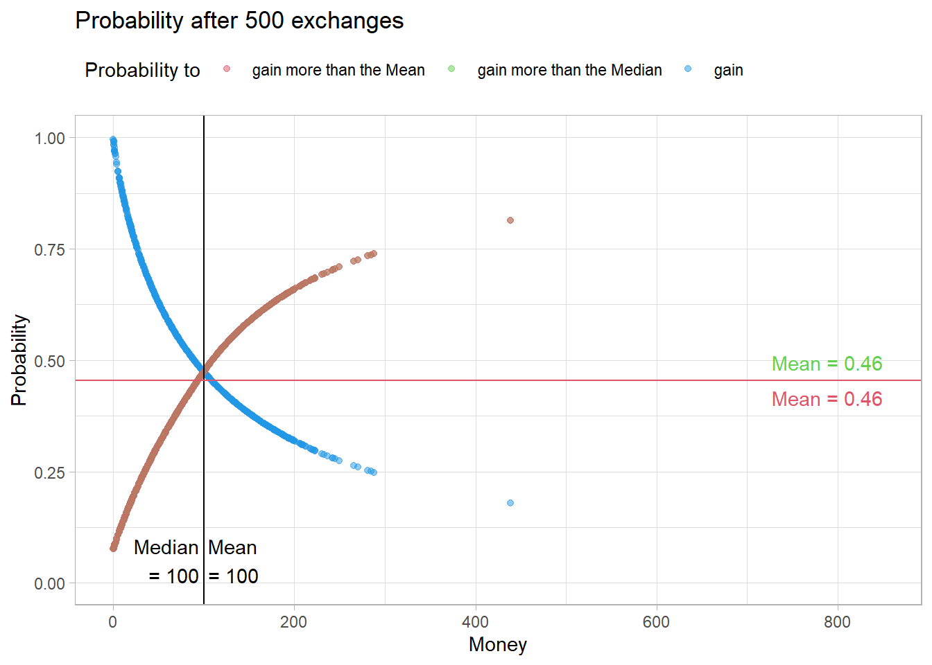

Therefore, the probability of meeting a rich agent in the future also decreases here. As a result, the probability of ending up above the median or the mean decreases here as well.

Fig11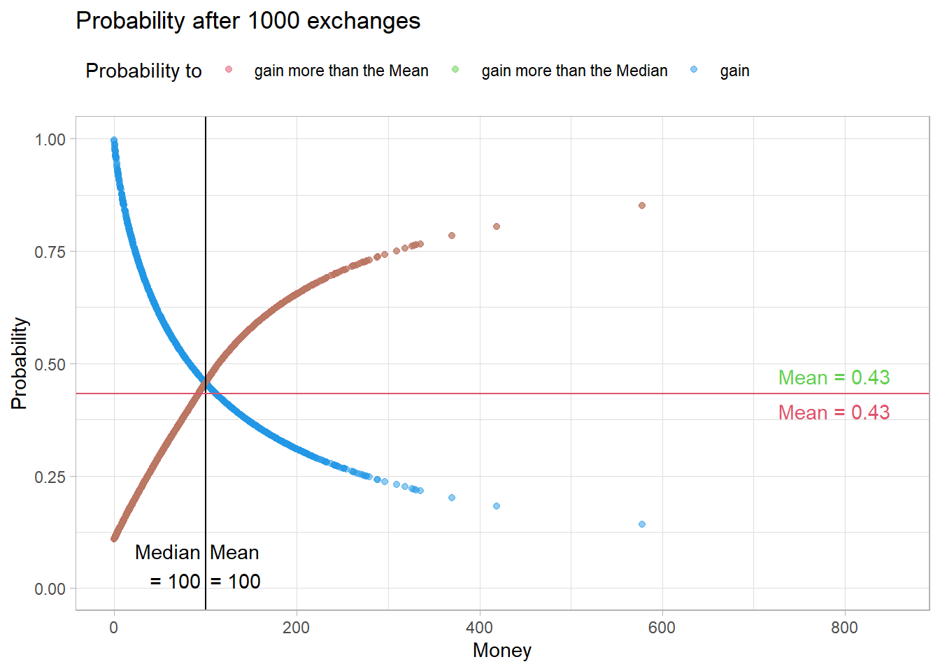

After 50000 meetings, the distribution of probabilities in this population looks almost identical.

Fig12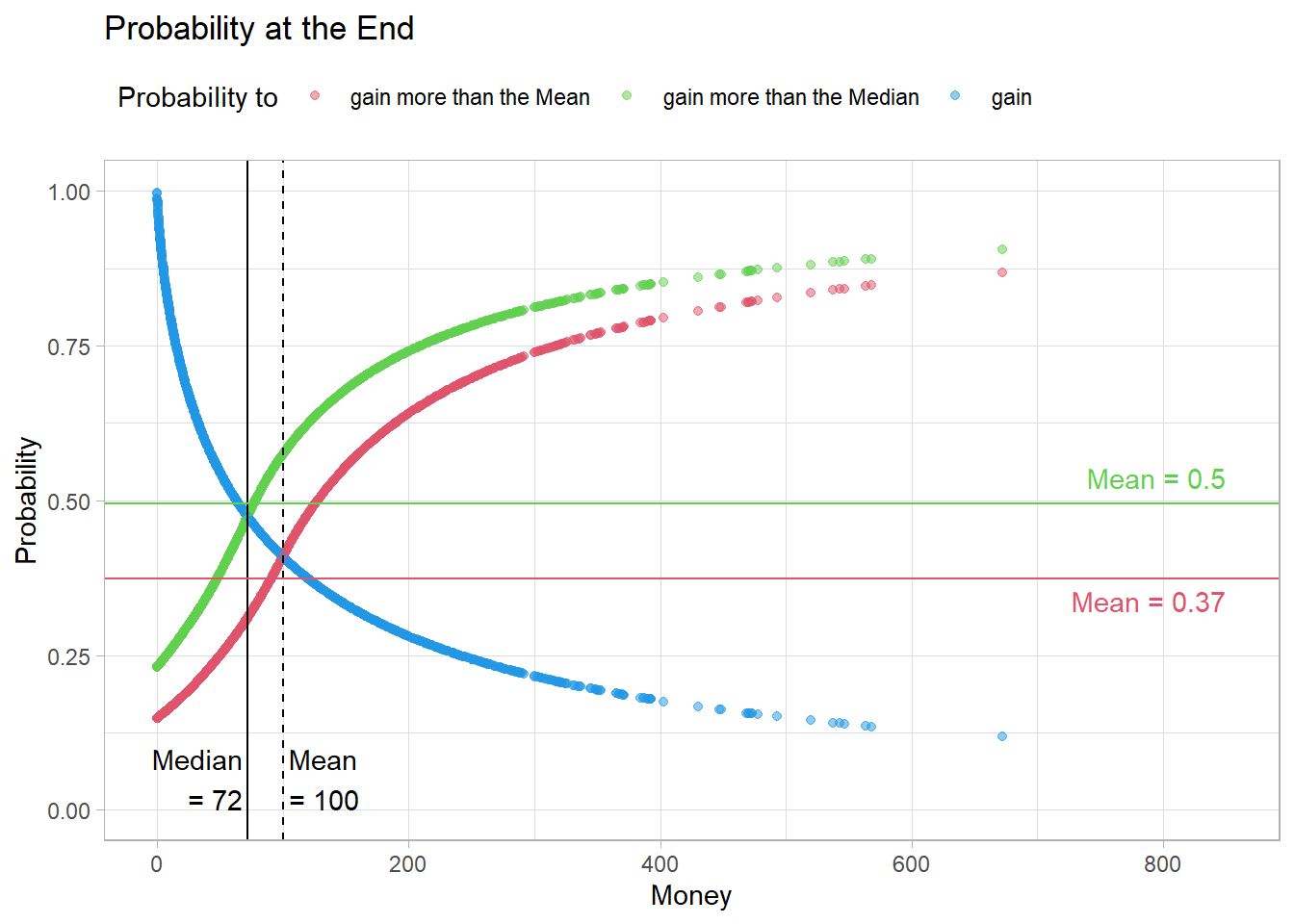

Probabilities over Time

This is even more evident over time.

ProbEqualt <- calc_p_t(eNorm$Timeline)

However, it seems that the median amount of money remains stable a bit longer.

Fig13 <- figProb_t(ProbEqualt, "Probability to ... of Money - Timeline")
Fig13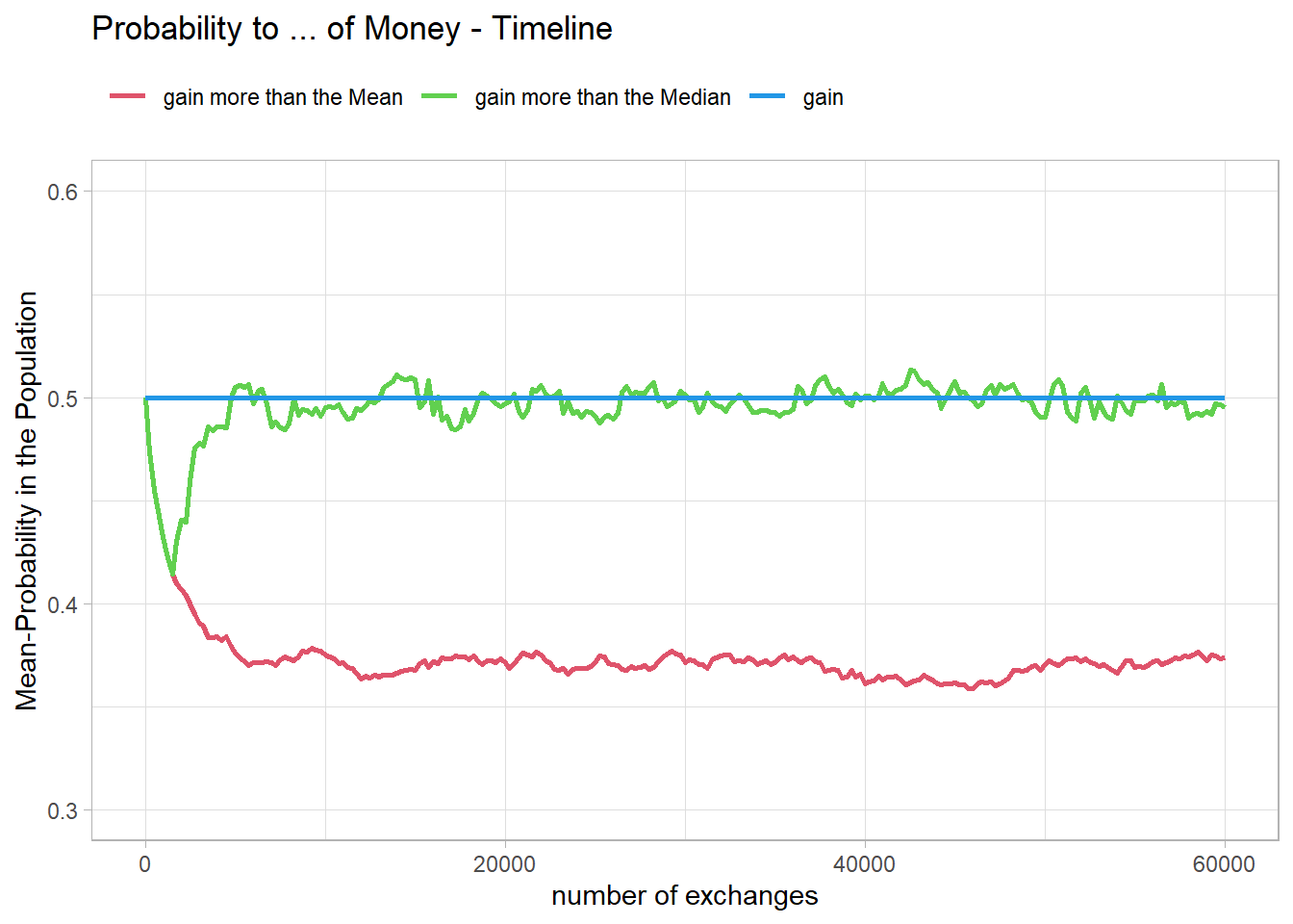

Comparison

To better compare the two populations, two new simulations are conducted. The number is restricted to the interesting initial range, and the time resolution is increased.

sNorms <- ecosim(8000, PopNorm$Money, TL = 50)
ProbNormts <- calc_p_t(sNorms$Timeline)
eNorms <- ecosim(8000, PopEqual$Money, TL = 50)
ProbEqualts <- calc_p_t(eNorms$Timeline)

Probabilities over Time

Fig14 <- figProb_t(ProbNormts, 
          "Probability to ... of Money\nTimeline for the Norm Population")
Fig15 <- figProb_t(ProbEqualts, 
          "Probability to ... of Money\nTimeline for a equal Population")

It actually shows that in the population with the normal distribution, the probabilities for the median and the mean separate earlier.

Fig14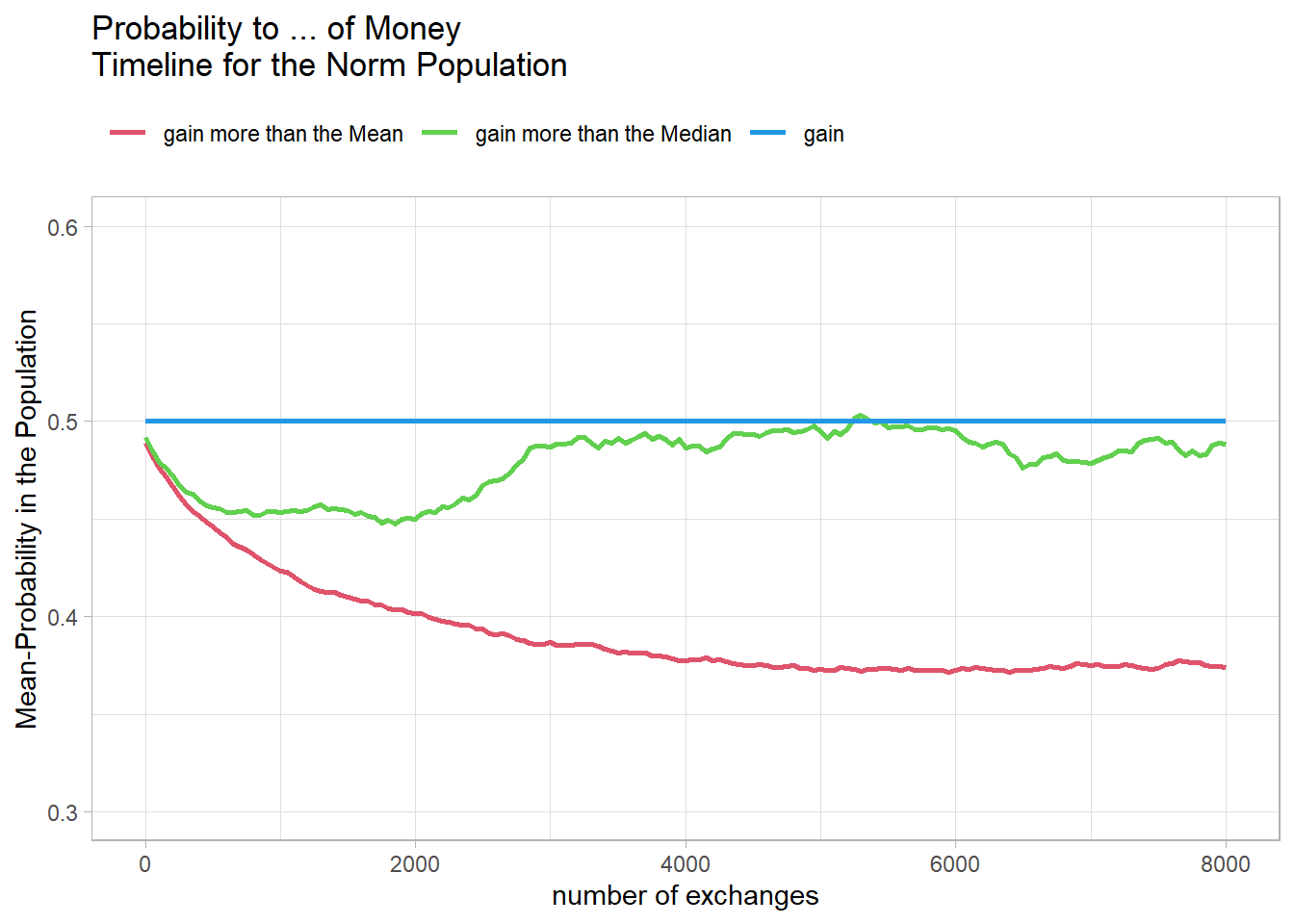

In the population with the same initial amount of money, the two lines remain very close together, meaning that the median and mean amounts of money remain almost identical.

Fig15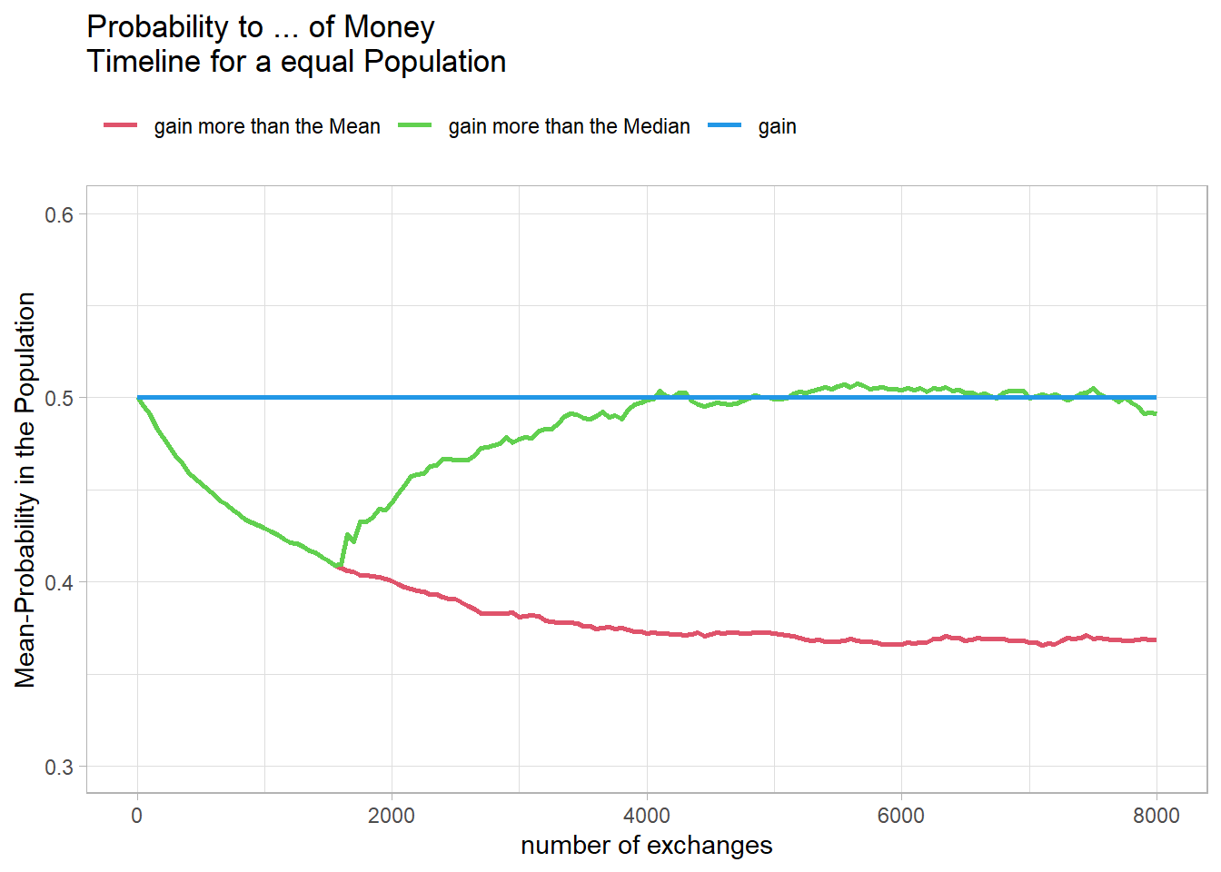

This makes sense because the meetings are random, and therefore some agents keep their starting balance of 100 longer. After 1500 meetings, or about two meetings per agent, this becomes increasingly unlikely.

Exploration

Since I have not yet used the Gini coefficient described in the article, it is now plotted over time for the two populations.

Fig16 <- data.frame( Time = ProbNormts[ProbNormts$Res == "Money",c("Time")],
                    Norm = gini_t(sNorms$Timeline),
                    Equal = gini_t(eNorms$Timeline)
                   )
Fig16 <- pivot_longer(data.frame(Fig16),
                      cols = !matches("Time"),
                      names_to = "Pop",
                      values_to = "Gini"
                      )
                    
Fig16p <- ggplot(data = Fig16, aes(x = Time, y = Gini, color = Pop)) +
  geom_line(linewidth = 1) +
  scale_color_manual(name = "Start Population", values = c(2, 1)) +
  ggtitle("Gini-Faktor - Timeline") +
  xlab("number of exchanges") +
  ylab("Gini") +
  theme_light() +
  theme(legend.position = "top",
        legend.justification = c(0, 1))

Fig16p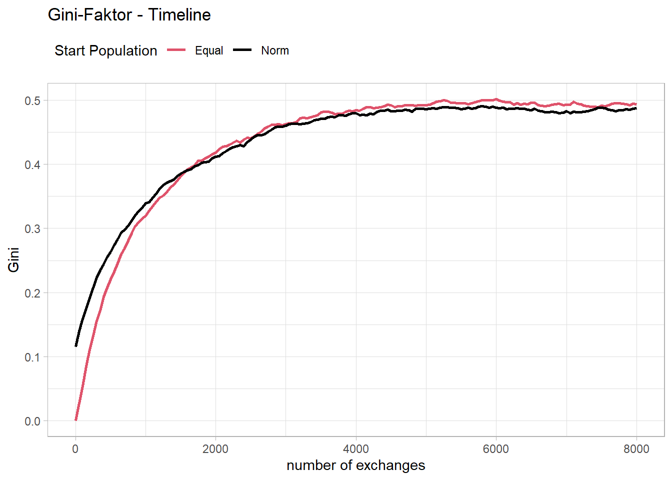

It seems that the course is quite similar to the course of the probability of ending up above the mean of the distribution. A closer look shows that the reciprocal of the Gini coefficient matches quite well with the probability of ending up above the mean of the distribution.

Fig17 <- data.frame( Time = ProbNormts[ProbNormts$Res == "Money",c("Time")],
                    GNorm = (1-Fig16[Fig16$Pop == "Norm","Gini"]),
                    PNorm = ProbNormts[ProbNormts$Res == "probmean",c("mean")],
                    GEqual = 1-Fig16[Fig16$Pop == "Equal","Gini"],
                    PEqual = ProbEqualts[ProbEqualts$Res == "probmean",c("mean")]
                   )
colnames(Fig17) <- c("Time", "GNorm", "PNorm", "GEqual", "PEqual")

Fig17$Faktn <- Fig17$GNorm/Fig17$PNorm
Fig17$Fakte <- Fig17$GEqual/Fig17$PEqual

Fig17 <- pivot_longer(data.frame(Fig17),
                      cols = starts_with("F"),
                      names_to = "Pop",
                      values_to = "Fakt"
                      )

Fig17p <- ggplot(data = Fig17, 
  aes(x = Time, y = Fakt, color = Pop, linetype = Pop)) +
  geom_line(linewidth = 1) +
  scale_color_manual(name = "Start Population", 
                     values = c(2, 1),
                     labels = c("Equal", "Norm")) +
  scale_linetype_manual("Start Population",
                        values = c("solid", "dashed"),
                        labels = c("Equal", "Norm")) +
  ggtitle("Relation between\n 
          Probability to gain more than the Mean\n
          and (1-Gini) - Timeline") +
  xlab("number of exchanges") +
  ylab("Faktor") +
  theme_light() +
  theme(legend.position = "top",
        legend.justification = c(0, 1))

Fig17p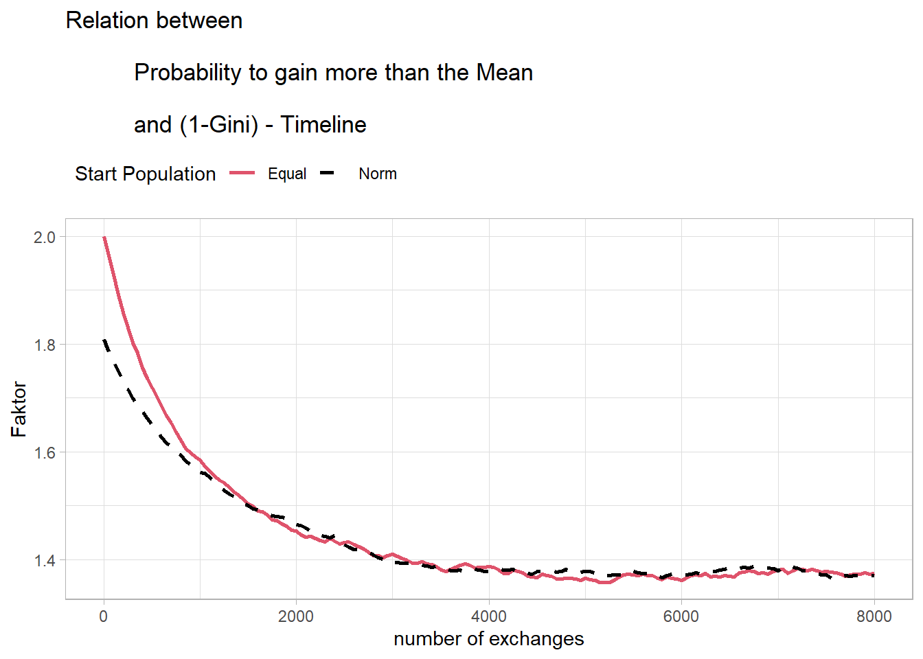

This could potentially allow for the development of a mathematical model for this mechanism. However, this exceeds my abilities and will be left to more capable individuals.

Numerical explanation

Minimal Population

To better illustrate the mechanism, I create a minimal population of three agents with a starting amount of 100.

set.seed(2)
PopMin <- rep(100,3)  
sMin <- ecosim(80, PopMin, TL = 1) 
sMint <- calc_p_t(sMin$Timeline) 
Fig18 <- figProb_t(sMint,"Probability to ... of Money\nTimeline for the Minimal Population") 
Fig18 

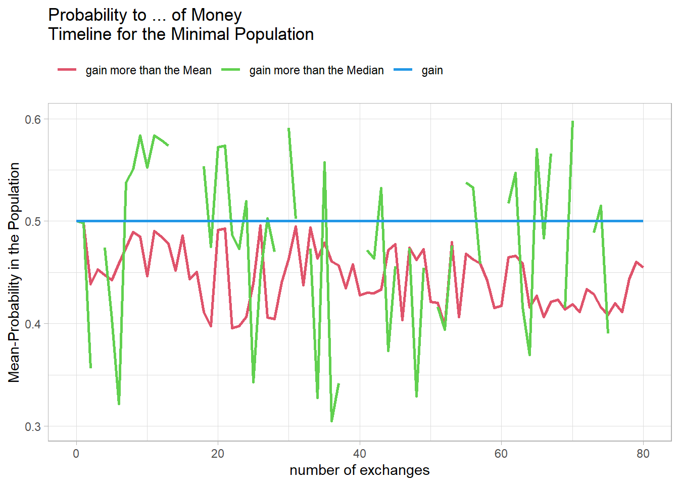
As you can see in Figure 18, the curves are very unstable, so I try a larger population with 5 agents.

set.seed(2)
PopMin <- rep(100,5)  
sMin <- ecosim(80, PopMin, TL = 1) 
sMint <- calc_p_t(sMin$Timeline) 
Fig19 <- figProb_t(sMint,"Probability to ... of Money\nTimeline for the Minimal Population") 
Fig19 

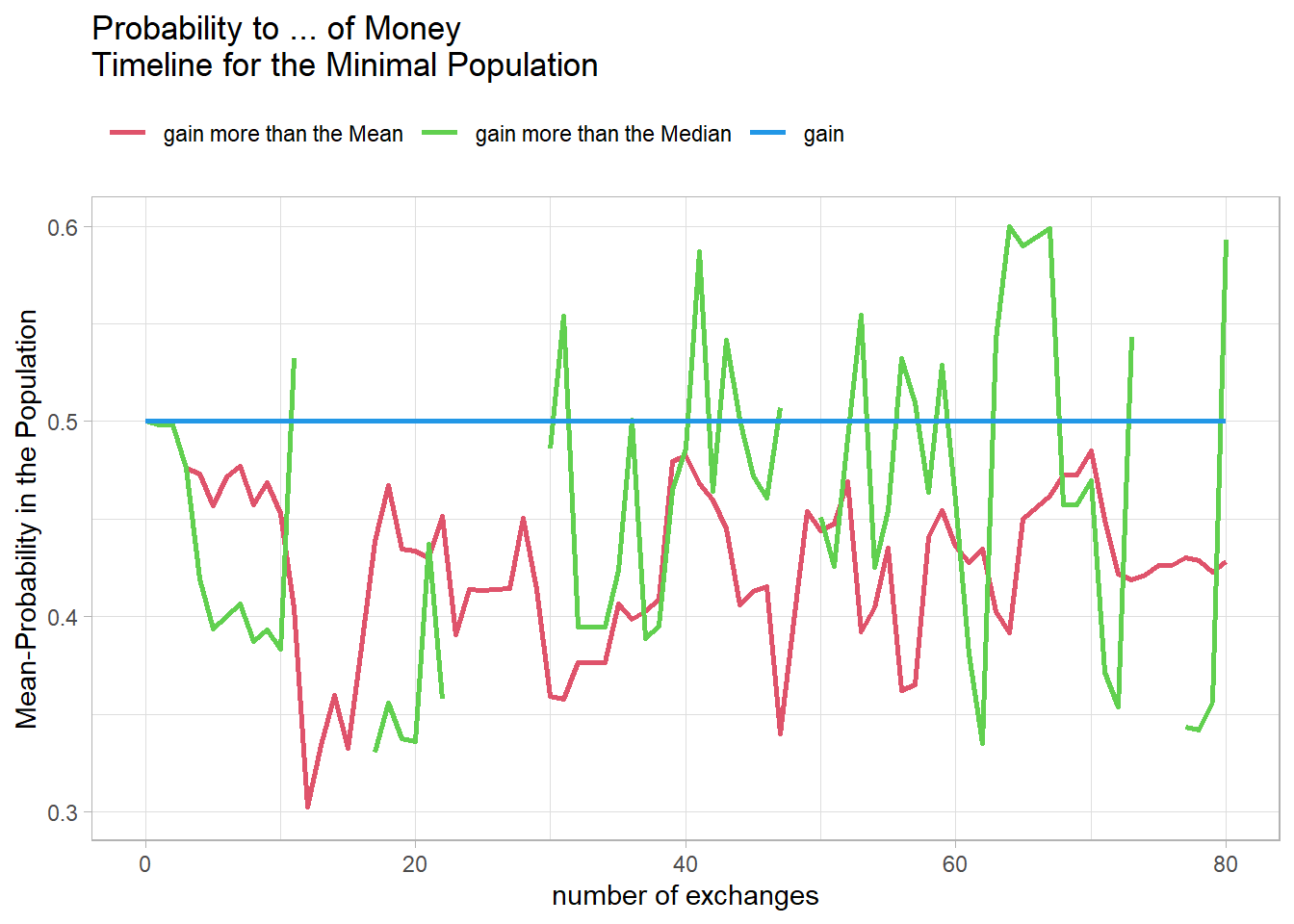
Here we still have the same problem, so the next time we double the number of agents to 10.

set.seed(2)
PopMin <- rep(100,10)  
sMin <- ecosim(80, PopMin, TL = 1) 
sMint <- calc_p_t(sMin$Timeline) 
Fig20 <- figProb_t(sMint,"Probability to ... of Money\nTimeline for the Minimal Population") 
Fig20 

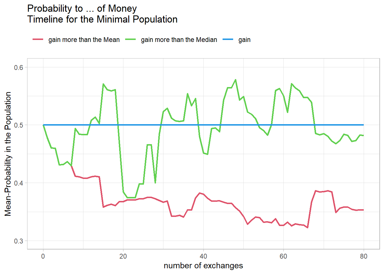
This seems to produce a reasonably stable curve. And this population is still small enough to make the tables clear. This is shown below for the start situation in Table1.

So all Probabilities for winning more than the median of Monay are exactly 0.5 unless which Agent is the next Meeting partner. The diagonals also show the mean scores for each agent in the given population.

ID	Money	Probabilities
		1	2	3	4	5	6	7	8	9	10
Money	100	100	100	100	100	100	100	100	100	100	100
1	100	0.5	0.5	0.5	0.5	0.5	0.5	0.5	0.5	0.5	0.5
2	100	0.5	0.5	0.5	0.5	0.5	0.5	0.5	0.5	0.5	0.5
3	100	0.5	0.5	0.5	0.5	0.5	0.5	0.5	0.5	0.5	0.5
4	100	0.5	0.5	0.5	0.5	0.5	0.5	0.5	0.5	0.5	0.5
5	100	0.5	0.5	0.5	0.5	0.5	0.5	0.5	0.5	0.5	0.5
6	100	0.5	0.5	0.5	0.5	0.5	0.5	0.5	0.5	0.5	0.5
7	100	0.5	0.5	0.5	0.5	0.5	0.5	0.5	0.5	0.5	0.5
8	100	0.5	0.5	0.5	0.5	0.5	0.5	0.5	0.5	0.5	0.5
9	100	0.5	0.5	0.5	0.5	0.5	0.5	0.5	0.5	0.5	0.5
10	100	0.5	0.5	0.5	0.5	0.5	0.5	0.5	0.5	0.5	0.5
Italic/bold = Median of Money, Bold = Mean in the Population

Table 1 clearly shows that the first money exchange does not only change the probability of the two affected agents. The other agents now also have the chance of meeting an agent with less money, which reduces the probability for all agents in the population.

ID	Money	Probabilities
		1	2	3	4	5	6	7	8	9	10
Money	100	100.0	100.0	100.0	100.0	33.6	166.4	100.0	100.0	100.0	100.0
1	100.0	0.49	0.50	0.50	0.50	0.25	0.62	0.50	0.50	0.50	0.50
2	100.0	0.50	0.49	0.50	0.50	0.25	0.62	0.50	0.50	0.50	0.50
3	100.0	0.50	0.50	0.49	0.50	0.25	0.62	0.50	0.50	0.50	0.50
4	100.0	0.50	0.50	0.50	0.49	0.25	0.62	0.50	0.50	0.50	0.50
5	33.6	0.25	0.25	0.25	0.25	0.28	0.50	0.25	0.25	0.25	0.25
6	166.4	0.62	0.62	0.62	0.62	0.50	0.61	0.62	0.62	0.62	0.62
7	100.0	0.50	0.50	0.50	0.50	0.25	0.62	0.49	0.50	0.50	0.50
8	100.0	0.50	0.50	0.50	0.50	0.25	0.62	0.50	0.49	0.50	0.50
9	100.0	0.50	0.50	0.50	0.50	0.25	0.62	0.50	0.50	0.49	0.50
10	100.0	0.50	0.50	0.50	0.50	0.25	0.62	0.50	0.50	0.50	0.49
Italic/bold = Median of Money, Bold = Mean in the Population

Until the 8th exchange The median and mean are exactly the same. (Table 2) As you can see, two agents still have the starting capital of 100. so the Median of Money is still 100.

ID	Money	Probabilities
		1	2	3	4	5	6	7	8	9	10
Money	100	196.6	40.6	64.2	100.0	33.6	190.9	136.3	130.4	7.4	100.0
1	196.6	0.64	0.58	0.62	0.66	0.57	0.74	0.70	0.69	0.51	0.66
2	40.6	0.58	0.29	0.05	0.29	0.00	0.57	0.43	0.42	0.00	0.29
3	64.2	0.62	0.05	0.34	0.39	0.00	0.61	0.50	0.49	0.00	0.39
4	100.0	0.66	0.29	0.39	0.44	0.25	0.66	0.58	0.57	0.07	0.50
5	33.6	0.57	0.00	0.00	0.25	0.27	0.55	0.41	0.39	0.00	0.25
6	190.9	0.74	0.57	0.61	0.66	0.55	0.63	0.69	0.69	0.50	0.66
7	136.3	0.70	0.43	0.50	0.58	0.41	0.69	0.54	0.63	0.30	0.58
8	130.4	0.69	0.42	0.49	0.57	0.39	0.69	0.63	0.52	0.27	0.57
9	7.4	0.51	0.00	0.00	0.07	0.00	0.50	0.30	0.27	0.19	0.07
10	100.0	0.66	0.29	0.39	0.50	0.25	0.66	0.58	0.57	0.07	0.44
Italic/bold = Median of Money, Bold = Mean in the Population

This is changing in the next steps (exchange 9 and 10) as seen in Table 3 and 4. Also to see there is that the median of Money falls down now and with this the probability to gain more than the median increases again.

The easiest way to see all this mechanistics is with Agent 10, who still has the starting amount of 100.

ID	Money	Probabilities
		1	2	3	4	5	6	7	8	9	10
Money	82.1	196.6	40.6	64.2	235.7	33.6	55.2	136.3	130.4	7.4	100.0
1	196.6	0.70	0.65	0.69	0.81	0.64	0.67	0.75	0.75	0.60	0.72
2	40.6	0.65	0.35	0.22	0.70	0.00	0.14	0.54	0.52	0.00	0.42
3	64.2	0.69	0.22	0.42	0.73	0.16	0.31	0.59	0.58	0.00	0.50
4	235.7	0.81	0.70	0.73	0.74	0.70	0.72	0.78	0.78	0.66	0.76
5	33.6	0.64	0.00	0.16	0.70	0.33	0.08	0.52	0.50	0.00	0.39
6	55.2	0.67	0.14	0.31	0.72	0.08	0.39	0.57	0.56	0.00	0.47
7	136.3	0.75	0.54	0.59	0.78	0.52	0.57	0.61	0.69	0.43	0.65
8	130.4	0.75	0.52	0.58	0.78	0.50	0.56	0.69	0.60	0.40	0.64
9	7.4	0.60	0.00	0.00	0.66	0.00	0.00	0.43	0.40	0.26	0.24
10	100.0	0.72	0.42	0.50	0.76	0.39	0.47	0.65	0.64	0.24	0.53
Italic/bold = Median of Money, Bold = Mean in the Population

ID	Money	Probabilities
		1	2	3	4	5	6	7	8	9	10
Money	82.1	196.6	40.6	64.2	235.7	33.6	3.4	136.3	182.2	7.4	100.0
1	196.6	0.69	0.65	0.69	0.81	0.64	0.59	0.75	0.78	0.60	0.72
2	40.6	0.65	0.35	0.22	0.70	0.00	0.00	0.54	0.63	0.00	0.42
3	64.2	0.69	0.22	0.39	0.73	0.16	0.00	0.59	0.67	0.00	0.50
4	235.7	0.81	0.70	0.73	0.73	0.70	0.66	0.78	0.80	0.66	0.76
5	33.6	0.64	0.00	0.16	0.70	0.34	0.00	0.52	0.62	0.00	0.39
6	3.4	0.59	0.00	0.00	0.66	0.00	0.27	0.41	0.56	0.00	0.21
7	136.3	0.75	0.54	0.59	0.78	0.52	0.41	0.60	0.74	0.43	0.65
8	182.2	0.78	0.63	0.67	0.80	0.62	0.56	0.74	0.68	0.57	0.71
9	7.4	0.60	0.00	0.00	0.66	0.00	0.00	0.43	0.57	0.28	0.24
10	100.0	0.72	0.42	0.50	0.76	0.39	0.21	0.65	0.71	0.24	0.51
Italic/bold = Median of Money, Bold = Mean in the Population

After 80 money exchanges, the median of the money takes on a kind of minimum. The probability of landing above the median is again 50% in the population. This is not quite correct, as Table 5 shows, because the simulation with only 10 agents is not very stable (Figure 20).

ID	Money	Probabilities
		1	2	3	4	5	6	7	8	9	10
Money	68.9	71.5	95.7	23.0	5.7	121.4	10.6	66.3	7.6	347.9	250.4
1	71.5	0.45	0.59	0.27	0.11	0.64	0.16	0.50	0.13	0.84	0.79
2	95.7	0.59	0.55	0.42	0.32	0.68	0.35	0.57	0.33	0.84	0.80
3	23.0	0.27	0.42	0.33	0.00	0.52	0.00	0.23	0.00	0.81	0.75
4	5.7	0.11	0.32	0.00	0.27	0.46	0.00	0.04	0.00	0.81	0.73
5	121.4	0.64	0.68	0.52	0.46	0.62	0.48	0.63	0.47	0.85	0.81
6	10.6	0.16	0.35	0.00	0.00	0.48	0.29	0.10	0.00	0.81	0.74
7	66.3	0.50	0.57	0.23	0.04	0.63	0.10	0.42	0.07	0.83	0.78
8	7.6	0.13	0.33	0.00	0.00	0.47	0.00	0.07	0.28	0.81	0.73
9	347.9	0.84	0.84	0.81	0.81	0.85	0.81	0.83	0.81	0.83	0.88
10	250.4	0.79	0.80	0.75	0.73	0.81	0.74	0.78	0.73	0.88	0.78
Italic/bold = Median of Money, Bold = Mean in the Population