tendencies <- 0.3
s_min <- max(1/tendencies,1/(1-tendencies))
s_min
[1] 3.333333var_max <- tendencies * (1-tendencies) / (s_min + 1)
var_max[1] 0.04846154This parameter describes the variance of the beta distribution. For mathematical reasons, the variance is defined relative to the maximum variance permitted for a given mean value. As a consequence, pvar is constrained to values greater than 0 and less than or equal to 1. This definition ensures that the resulting beta distribution parameters are always greater than 1, and that the mode of the distribution lies within the interval (0,1).
tendencies <- 0.3
s_min <- max(1/tendencies,1/(1-tendencies))
s_min[1] 3.333333var_max <- tendencies * (1-tendencies) / (s_min + 1)
var_max[1] 0.04846154Formally, pvar is defined as follows:
Finally, this formulation makes it possible to derive a precision parameter and, based on it, the corresponding beta distribution parameters from only two inputs (Tendency, pvar)
calc_beta_par <- function(tendencies, pvar, output = NULL, eps = 1e-6) {
    len <- length(tendencies * pvar)
    df <- data.frame(ten = rep(0, len))

    df$ten <- pmin(pmax(tendencies, eps), 1 - eps)
    df$pvar <- pmax(pmin(pvar, 2), eps)

    df$ab_min <- pmax(1/df$ten,1/(1-df$ten))
    df$var_max <- df$ten * (1 - df$ten) / (df$ab_min + 1)

    df$var <- df$pvar * df$var_max

    df$prec <- (df$ten * (1 - df$ten)) / df$var - 1

    df$a <- df$prec * df$ten
    df$b <- df$prec * (1 - df$ten)

    if (is.null(output)) {
        return(df)
    } else {
        missing <- setdiff(output, colnames(df))
        if (length(missing) > 0) {
            stop("Unknown output columns: ", paste(missing, collapse = ", "))
        } else {
            df[, output]
        }
    }
}

calc_beta_par(c(0.1, 0.3, 0.5, 0.7, 0.9), 1)
ten pvar ab_min var_max var prec a b
1 0.1 1 10.000000 0.008181818 0.008181818 10.000000 1.000000 9.000000
2 0.3 1 3.333333 0.048461538 0.048461538 3.333333 1.000000 2.333333
3 0.5 1 2.000000 0.083333333 0.083333333 2.000000 1.000000 1.000000
4 0.7 1 3.333333 0.048461538 0.048461538 3.333333 2.333333 1.000000
5 0.9 1 10.000000 0.008181818 0.008181818 10.000000 9.000000 1.000000calc_beta_par(c(0.1, 0.3, 0.5, 0.7, 0.9), 0.5) ten pvar ab_min var_max var prec a b
1 0.1 0.5 10.000000 0.008181818 0.004090909 21.000000 2.100000 18.900000
2 0.3 0.5 3.333333 0.048461538 0.024230769 7.666667 2.300000 5.366667
3 0.5 0.5 2.000000 0.083333333 0.041666667 5.000000 2.500000 2.500000
4 0.7 0.5 3.333333 0.048461538 0.024230769 7.666667 5.366667 2.300000
5 0.9 0.5 10.000000 0.008181818 0.004090909 21.000000 18.900000 2.100000calc_beta_par(c(0.1, 0.3, 0.5, 0.7, 0.9), 0) ten pvar ab_min var_max var prec a b
1 0.1 1e-06 10.000000 0.008181818 8.181818e-09 10999999 1100000 9899999
2 0.3 1e-06 3.333333 0.048461538 4.846154e-08 4333332 1300000 3033333
3 0.5 1e-06 2.000000 0.083333333 8.333333e-08 2999999 1500000 1500000
4 0.7 1e-06 3.333333 0.048461538 4.846154e-08 4333332 3033333 1300000
5 0.9 1e-06 10.000000 0.008181818 8.181818e-09 10999999 9899999 1100000calc_beta_par(c(0.1, 0.3, 0.5, 0.7, 0.9), 2) ten pvar ab_min var_max var prec a b
1 0.1 2 10.000000 0.008181818 0.01636364 4.500000 0.4500000 4.0500000
2 0.3 2 3.333333 0.048461538 0.09692308 1.166667 0.3500000 0.8166667
3 0.5 2 2.000000 0.083333333 0.16666667 0.500000 0.2500000 0.2500000
4 0.7 2 3.333333 0.048461538 0.09692308 1.166667 0.8166667 0.3500000
5 0.9 2 10.000000 0.008181818 0.01636364 4.500000 4.0500000 0.4500000Function that calculates the frequency distribution and the probability distribution for each value of x, for all given parameter sets (tendencies and pvar).
features_dist <- function(x, tendencies, pvar, output = NULL, eps = 1e-6) {
    par <- calc_beta_par(tendencies, pvar, output = c("a","b"), eps)
    lenpar <- length(par$a)
    lenx <- length(x)
    df <- data.frame(
        set = rep(1:lenpar, each = lenx),
        x = rep(x,lenpar),
        a = rep(par$a, each = lenx),
        b = rep(par$b, each = lenx)
    )
    df$freq <- dbeta(df$x, df$a, df$b)
    df$mode <- (df$a - 1) / (df$a + df$b - 2)
    df$mode <- pmin(pmax(df$mode, 0), 1)
    df$max <- ifelse(is.na(df$mode),
                     df$freq,
                     dbeta(df$mode, df$a, df$b))
    df$probx <- df$freq / df$max
    df$prob <- pbeta(df$x, df$a, df$b)

    if (is.null(output)) {
        return(df)
    } else {
        missing <- setdiff(output, colnames(df))
        if (length(missing) > 0) {
            stop("Unknown output columns: ", paste(missing, collapse = ", "))
        } else {
            df[, output]
        }
    }
}

features_dist(x = c(0, 0.5, 1),
              tendencies = 0.6,
              pvar = 1)
set x a b freq mode max probx prob
1 1 0.0 1.5 1 0.00000 1 Inf 0 0.0000000
2 1 0.5 1.5 1 1.06066 1 Inf 0 0.3535534
3 1 1.0 1.5 1 Inf 1 Inf NaN 1.0000000features_dist(x = c(0, 0.5, 1),
tendencies = c(0.3, 0.5, 0.7),
pvar = 0.5,
output = c("set", "freq", "prob", "probx")) set freq prob probx
1 1 0.000000 0.000000 0.0000000
2 1 1.034560 0.883187 0.4164587
3 1 0.000000 1.000000 0.0000000
4 2 0.000000 0.000000 0.0000000
5 2 1.697653 0.500000 1.0000000
6 2 0.000000 1.000000 0.0000000
7 3 0.000000 0.000000 0.0000000
8 3 1.034560 0.116813 0.4164587
9 3 0.000000 1.000000 0.0000000The following plot illustrates the preference distribution for a specific feature. The x-axis represents the cognitively interpreted expression of the feature, while the y-axis depicts the corresponding preference. Accordingly, the curve reaches its maximum at the point where the individual feels most comfortable.
plot_features_dist(tendencies = c(0.1, 0.2, 0.3, 0.4, 0.5, 0.6, 0.7, 0.8, 0.9),
                   pvar = 0.5,
                   title ="Preference distribution for a feature across different tendencies (pvar = 0.5)")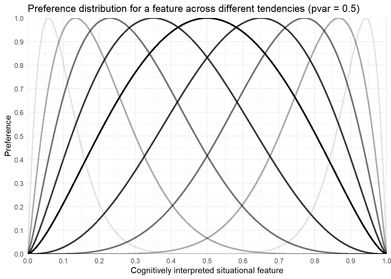
In the following special case, a “maximum” variation is assumed (pvar = 1). As can be seen, a tendency of 0.5 results in a nearly uniform distribution. This can be interpreted as indifference with respect to this feature.
plot_features_dist(tendencies = c(0.4, 0.45, 0.5, 0.55, 0.6),
                   pvar = 1,
                   title ="Preference distribution for a feature across different tendencies (pvar = 1)")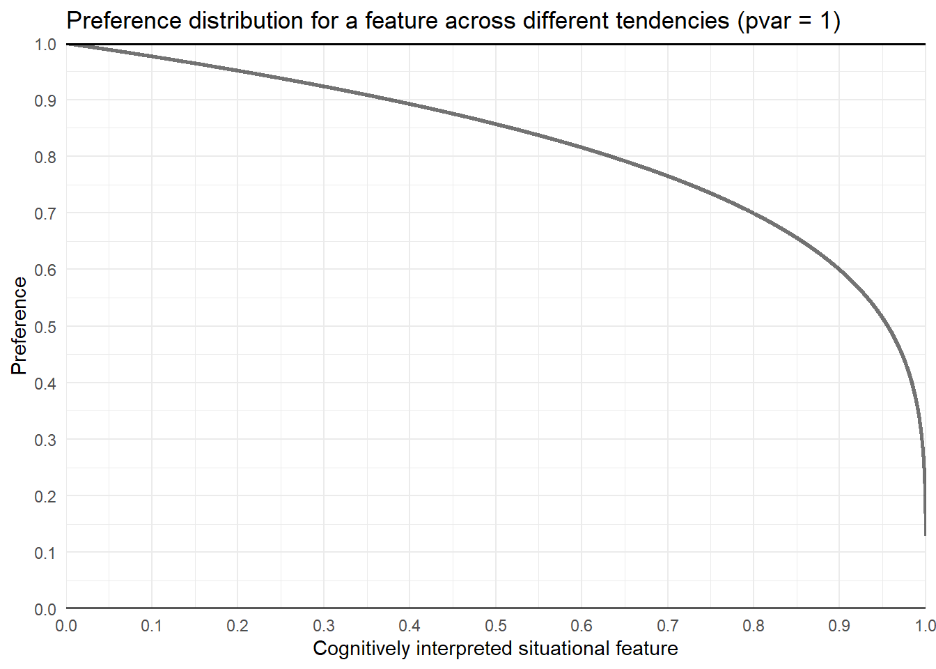
features_dist <- function(x, tendencies, pvar, output = NULL, eps = 1e-6) {
    par <- calc_beta_par(tendencies, pvar, output = c("a", "b", "pvar"), eps)
    lenpar <- length(par$a)
    lenx <- length(x)
    df <- data.frame(
        set = rep(1:lenpar, each = lenx),
        x = rep(x,lenpar),
        a = rep(par$a, each = lenx),
        b = rep(par$b, each = lenx),
        pvar = rep(par$pvar, each = lenx)
    )
    df$freq <- dbeta(df$x, df$a, df$b)
    df$prob <- pbeta(df$x, df$a, df$b)
    df$probx <- df$freq / (1 + df$freq)

    if (is.null(output)) {
        return(df)
    } else {
        missing <- setdiff(output, colnames(df))
        if (length(missing) > 0) {
            stop("Unknown output columns: ", paste(missing, collapse = ", "))
        } else {
            df[, output]
        }
    }
}plot_features_dist(tendencies = c(0.1, 0.2, 0.3, 0.4, 0.5, 0.6, 0.7, 0.8, 0.9),
pvar = 0.5,
title ="Preference distribution for a feature across different tendencies (pvar = 0.5)",
save = "Features")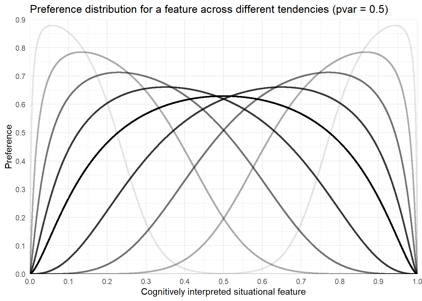
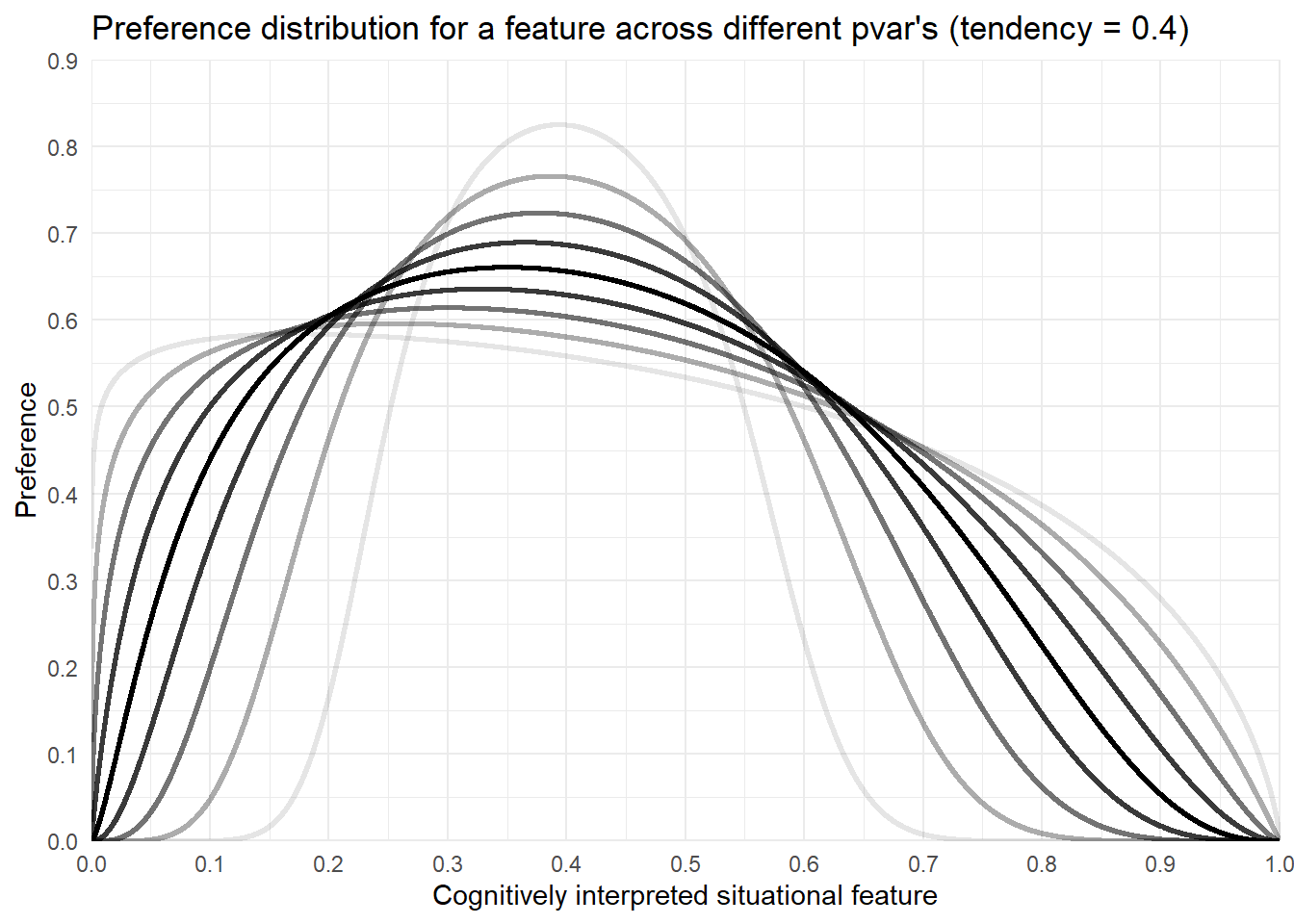
plot_features_dist(tendencies = 0.4,
                   pvar = c(0.1, 0.2, 0.3, 0.4, 0.5, 0.6, 0.7, 0.8, 0.9),
                   title ="Preference distribution for a feature across different pvar's (tendency = 0.4)")