---
title: "Cognitive Bias"
author: "Hubert Bächli"
date: last-modified
---
```{r setup, include=FALSE}
knitr::opts_chunk$set(echo = TRUE)
library(here)
library(tidyverse)
calc_beta_par <- function(tendencies, pvar, output = NULL, eps = 1e-6) {
len <- length(tendencies * pvar)
df <- data.frame(ten = rep(0, len))
df$ten <- pmin(pmax(tendencies, eps), 1 - eps)
df$pvar <- pmax(pmin(pvar, 2), eps)
df$ab_min <- pmax(1/df$ten,1/(1-df$ten))
df$var_max <- df$ten * (1 - df$ten) / (df$ab_min + 1)
df$var <- df$pvar * df$var_max
df$prec <- (df$ten * (1 - df$ten)) / df$var - 1
df$a <- df$prec * df$ten
df$b <- df$prec * (1 - df$ten)
if (is.null(output)) {
return(df)
} else {
missing <- setdiff(output, colnames(df))
if (length(missing) > 0) {
stop("Unknown output columns: ", paste(missing, collapse = ", "))
} else {
df[, output]
}
}
}
features_dist <- function(x, tendencies, pvar, output = NULL, eps = 1e-6) {
par <- calc_beta_par(tendencies, pvar, output = c("a","b"), eps)
lenpar <- length(par$a)
lenx <- length(x)
df <- data.frame(
set = rep(1:lenpar, each = lenx),
x = rep(x,lenpar),
a = rep(par$a, each = lenx),
b = rep(par$b, each = lenx)
)
df$freq <- dbeta(df$x, df$a, df$b)
df$mode <- (df$a - 1) / (df$a + df$b - 2)
df$mode <- pmin(pmax(df$mode, 0), 1)
df$max <- ifelse(is.na(df$mode),
df$freq,
dbeta(df$mode, df$a, df$b))
df$probx <- df$freq / df$max
df$prob <- pbeta(df$x, df$a, df$b)
if (is.null(output)) {
return(df)
} else {
missing <- setdiff(output, colnames(df))
if (length(missing) > 0) {
stop("Unknown output columns: ", paste(missing, collapse = ", "))
} else {
df[, output]
}
}
}
```
# Cognitive Bias
## Definitions
```{r}
cog_bias_m <- 0.2 # mean shift
cog_bias_v <- 1.2 # factor for pvar
```
## Updating Cognitive Bias
The cognitive bias can either be defined a priori or dynamically updated throughout the simulation as a function of the accumulated experiences.
```{r}
obj_mean <- 0.4
obj_pvar <- 0.4
cog_mean <- 0.6
cog_pvar <- 0.5
```
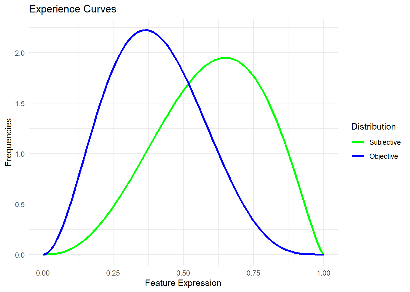
These given curve parameters define the cognitive bias.
```{r}
cog_bias_m <- obj_mean - cog_mean
cog_bias_m
cog_bias_v <- obj_pvar / cog_pvar
cog_bias_v
```
## Visualisation
```{r, echo = FALSE}
n <- 100
x <- seq(0, 1, length.out = n)
df <- data.frame(
x = x,
obj_dist = features_dist(x, obj_mean, obj_pvar, output = c("freq")),
obj_prob = features_dist(x, obj_mean, obj_pvar, output = c("prob")),
cog_dist = features_dist(x, cog_mean, cog_pvar, output = c("freq")),
cog_prob = features_dist(x, cog_mean, cog_pvar, output = c("prob"))
)
df_long <- df %>%
pivot_longer(
cols = -x,
names_to = c("type", "curve"),
names_sep = "_",
values_to = "value"
)
```
```{r, echo = FALSE}
ggplot(
df_long %>% filter(curve == "dist"),
aes(x = x, y = value, color = type)
) +
geom_line(linewidth = 1.2) +
scale_color_manual(
values = c(
"obj" = "blue",
"cog" = "green"
),
labels = c(
"obj" = "Objective",
"cog" = "Subjective"
)
) +
labs(
x = "Feature Expression",
y = "Frequencies",
color = "Distribution",
title = "Experience Curves"
) +
theme_minimal()
```
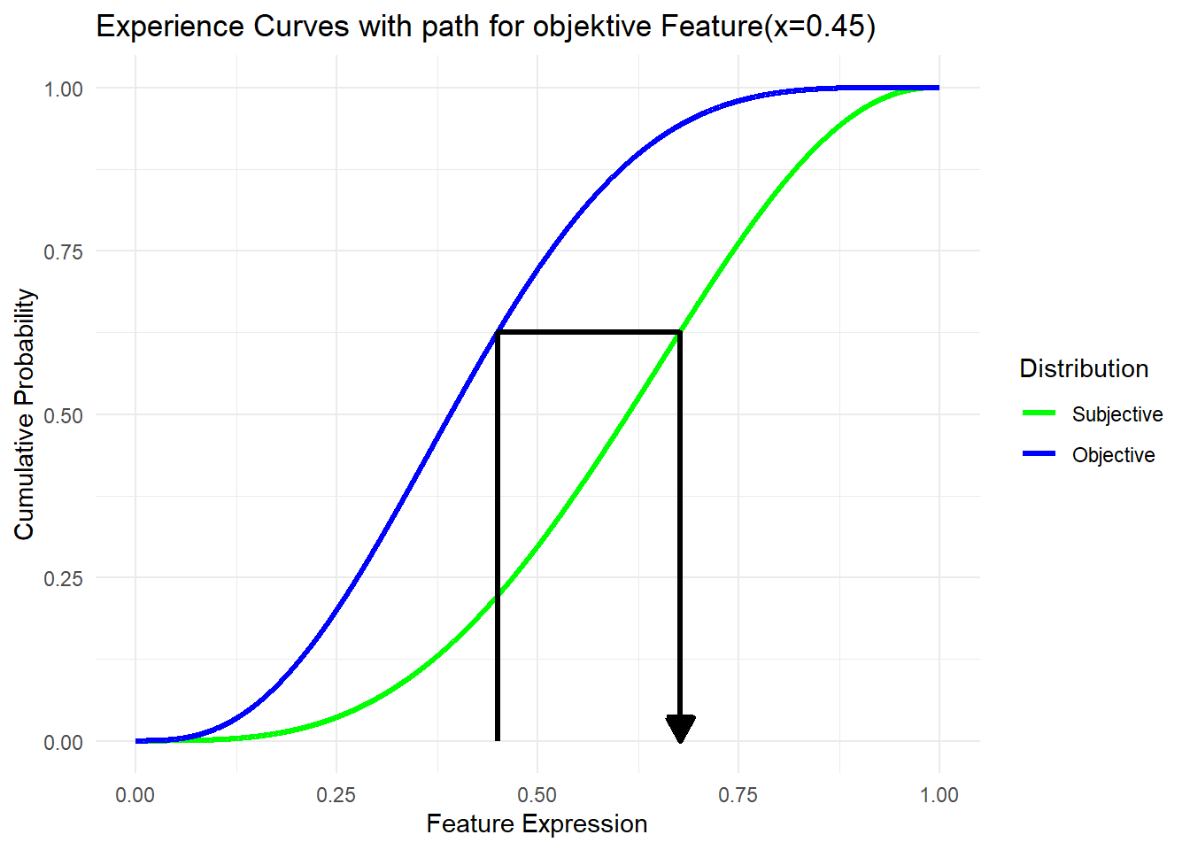
```{r, echo = FALSE}
plot_cog_bias <- function(path, obj_mean, obj_pvar, cog_mean, cog_pvar, title, save = NULL) {
x <- seq(0, 1, 0.0001)
df <- data.frame(
x = x,
obj_dist = features_dist(x, obj_mean, obj_pvar, output = c("freq")),
obj_prob = features_dist(x, obj_mean, obj_pvar, output = c("prob")),
cog_dist = features_dist(x, cog_mean, cog_pvar, output = c("freq")),
cog_prob = features_dist(x, cog_mean, cog_pvar, output = c("prob"))
) %>%
pivot_longer(
cols = -x,
names_to = c("type", "curve"),
names_sep = "_",
values_to = "value"
) %>%
filter(curve == "prob")
px1 <- path
py1 <- 0
py2 <- features_dist(path, obj_mean, obj_pvar, output = c("prob"))
par <- calc_beta_par(cog_mean, cog_pvar, output = c("a","b"))
px2 <- qbeta(py2, par$a, par$b)
path_df <- data.frame(
x = c(px1, px1, px2, px2),
y = c(py1, py2, py2, py1)
)
plt <- ggplot(
df, aes(x = x, y = value, color = type)) +
geom_line(linewidth = 1.2) +
scale_color_manual(
values = c("obj" = "blue",
"cog" = "green"),
labels = c("obj" = "Objective",
"cog" = "Subjective")) +
geom_line(data = path_df,
aes(x = x, y = y),
linewidth = 1.2,
inherit.aes = FALSE,
color = "black",
arrow = arrow(type = "closed",
length = unit(4, "mm"))) +
labs(x = "Feature Expression",
y = "Cumulative Probability",
color = "Distribution",
title = title ) +
theme_minimal()
if (!is.null(save)) {
dir_path <- "img"
dir.create(dir_path, recursive = TRUE, showWarnings = FALSE)
file_path <- file.path(dir_path, paste0(save, ".png"))
ggsave(filename = file_path,
plot = plt,
width = 8,
height = 4,
units = "in",
dpi = 300)
}
plt
}
```
```{r}
plot_cog_bias(0.45,
              obj_mean, obj_pvar,
              cog_mean, cog_pvar,
              title = "Experience Curves with path for objektive Feature(x=0.45)",
              save = "Cognitive_Bias")
```
# \< [Back](../Personality.qmd#cog_bias)