---
title: "Aggregating Fasets and Traits"
author: "Hubert Bächli"
date: last-modified
---
```{r setup, include=FALSE}
knitr::opts_chunk$set(echo = TRUE)
library(here)
library(tidyverse)
calc_beta_par <- function(tendencies, pvar, output = NULL, eps = 1e-6) {
len <- length(tendencies * pvar)
df <- data.frame(ten = rep(0, len))
df$ten <- pmin(pmax(tendencies, eps), 1 - eps)
df$pvar <- pmax(pmin(pvar, 2), eps)
df$ab_min <- pmax(1/df$ten,1/(1-df$ten))
df$var_max <- df$ten * (1 - df$ten) / (df$ab_min + 1)
df$var <- df$pvar * df$var_max
df$prec <- (df$ten * (1 - df$ten)) / df$var - 1
df$a <- df$prec * df$ten
df$b <- df$prec * (1 - df$ten)
if (is.null(output)) {
return(df)
} else {
missing <- setdiff(output, colnames(df))
if (length(missing) > 0) {
stop("Unknown output columns: ", paste(missing, collapse = ", "))
} else {
df[, output]
}
}
}
features_dist <- function(x, tendencies, pvar, output = NULL, eps = 1e-6) {
par <- calc_beta_par(tendencies, pvar, output = c("a","b"), eps)
lenpar <- length(par$a)
lenx <- length(x)
df <- data.frame(
set = rep(1:lenpar, each = lenx),
x = rep(x,lenpar),
a = rep(par$a, each = lenx),
b = rep(par$b, each = lenx)
)
df$freq <- dbeta(df$x, df$a, df$b)
df$mode <- (df$a - 1) / (df$a + df$b - 2)
df$mode <- pmin(pmax(df$mode, 0), 1)
df$max <- ifelse(is.na(df$mode),
df$freq,
dbeta(df$mode, df$a, df$b))
df$probx <- df$freq / df$max
df$prob <- pbeta(df$x, df$a, df$b)
if (is.null(output)) {
return(df)
} else {
missing <- setdiff(output, colnames(df))
if (length(missing) > 0) {
stop("Unknown output columns: ", paste(missing, collapse = ", "))
} else {
df[, output]
}
}
}
plot_features_dist <- function(tendencies, pvar, title, save = NULL) {
x <- seq(0, 1, 0.0001)
len <- length(tendencies * pvar)
df <- features_dist(
x = x,
tendencies = tendencies,
pvar = pvar
)
df$alpha <- 0.3
plt <- ggplot(
df, aes( x = x, y = probx, group = set)) +
geom_line(aes(alpha = alpha), linewidth = 1) +
scale_alpha_identity() +
labs(
x = "Cognitively interpreted situational feature",
y = "Preference",
title = title
) +
theme_minimal()
if (!is.null(save)) {
dir_path <- "img"
dir.create(dir_path, recursive = TRUE, showWarnings = FALSE)
file_path <- file.path(dir_path, paste0(save, ".png"))
ggsave(filename = file_path,
plot = plt,
width = 8,
height = 4,
units = "in",
dpi = 300)
}
plt
}
```
# Aggregating Fasets and Traits
## Example
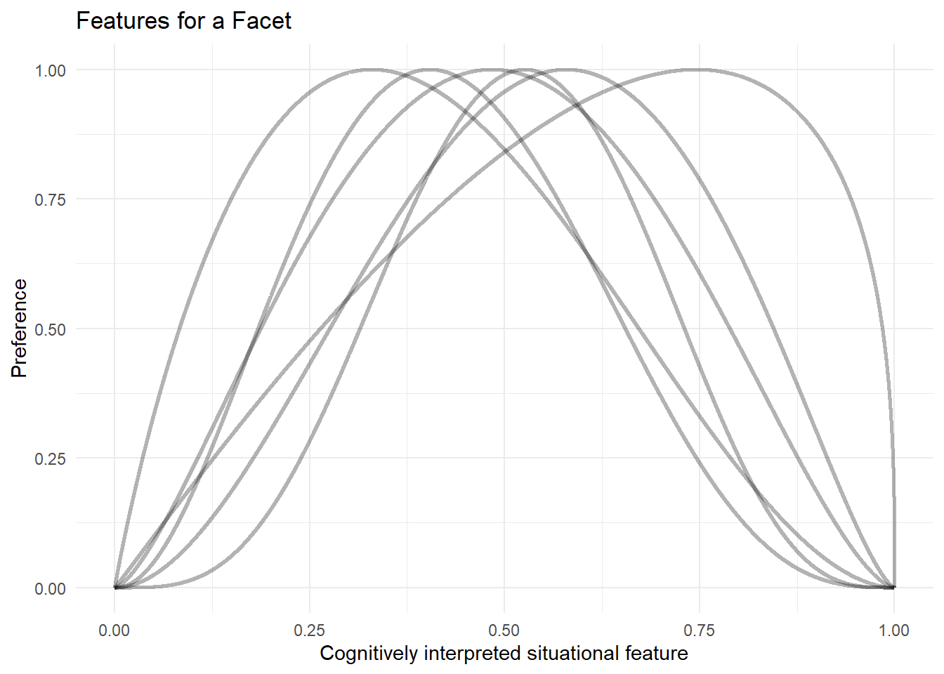
### 1
```{r}
tendencies_1 <- c(0.4, 0.43, 0.49, 0.52, 0.55, 0.6)
pvar_1 <- c(0.6, 0.4, 0.5, 0.3, 0.5, 0.8)
```
```{r}
x <- seq(0, 1, 0.001)
df_1 <- features_dist(x, tendencies_1, pvar_1)
head(df_1)
plot_features_dist(tendencies_1, pvar_1, "Features for a Facet")
```
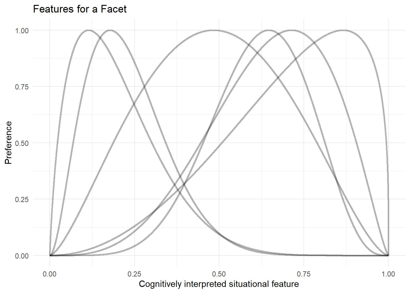
### 2
```{r}
tendencies_2 <- c(0.2, 0.23, 0.49, 0.62, 0.65, 0.7)
pvar_2 <- c(0.6, 0.4, 0.5, 0.3, 0.5, 0.8)
```
```{r}
x <- seq(0, 1, 0.001)
df_2 <- features_dist(x, tendencies_2, pvar_2)
head(df_2)
plot_features_dist(tendencies_2, pvar_2, "Features for a Facet")
```
## Aggregating
```{r}
facets_1 <- df_1 %>%
    group_by(x) %>%
    summarise(
    a = mean(a),
    b = mean(b),
    probx = mean(probx),
    .groups = "drop"
    )

head(facets_1)
```
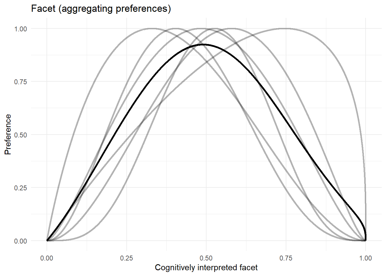
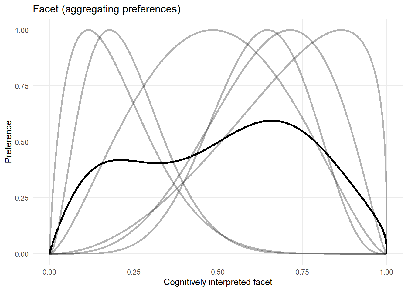
## Aggregating preferences
```{r, echo = FALSE}
plot_facet_pref <- function(tendencies, pvar, title, save = NULL) {
x <- seq(0, 1, 0.0001)
len <- length(tendencies * pvar)
df <- features_dist(
x = x,
tendencies = tendencies,
pvar = pvar
)
df$alpha <- 0.3
facet <- df %>%
group_by(x) %>%
summarise(
probx = mean(probx),
.groups = "drop"
)
plt <- ggplot(
df, aes( x = x, y = probx, group = set)) +
geom_line(aes(alpha = alpha), linewidth = 1) +
scale_alpha_identity() +
geom_line(
data = facet,
aes(x = x, y = probx),
inherit.aes = FALSE,
linewidth = 1.2,
color = "black" ) +
labs(
x = "Cognitively interpreted facet",
y = "Preference",
title = title ) +
theme_minimal()
if (!is.null(save)) {
dir_path <- "img"
dir.create(dir_path, recursive = TRUE, showWarnings = FALSE)
file_path <- file.path(dir_path, paste0(save, ".png"))
ggsave(filename = file_path,
plot = plt,
width = 8,
height = 4,
units = "in",
dpi = 300)
}
plt
}
```
```{r}
plot_facet_pref(tendencies_1, pvar_1, "Facet (aggregating preferences)")
plot_facet_pref(tendencies_2, pvar_2, "Facet (aggregating preferences)", save = "Facet_pref")
```
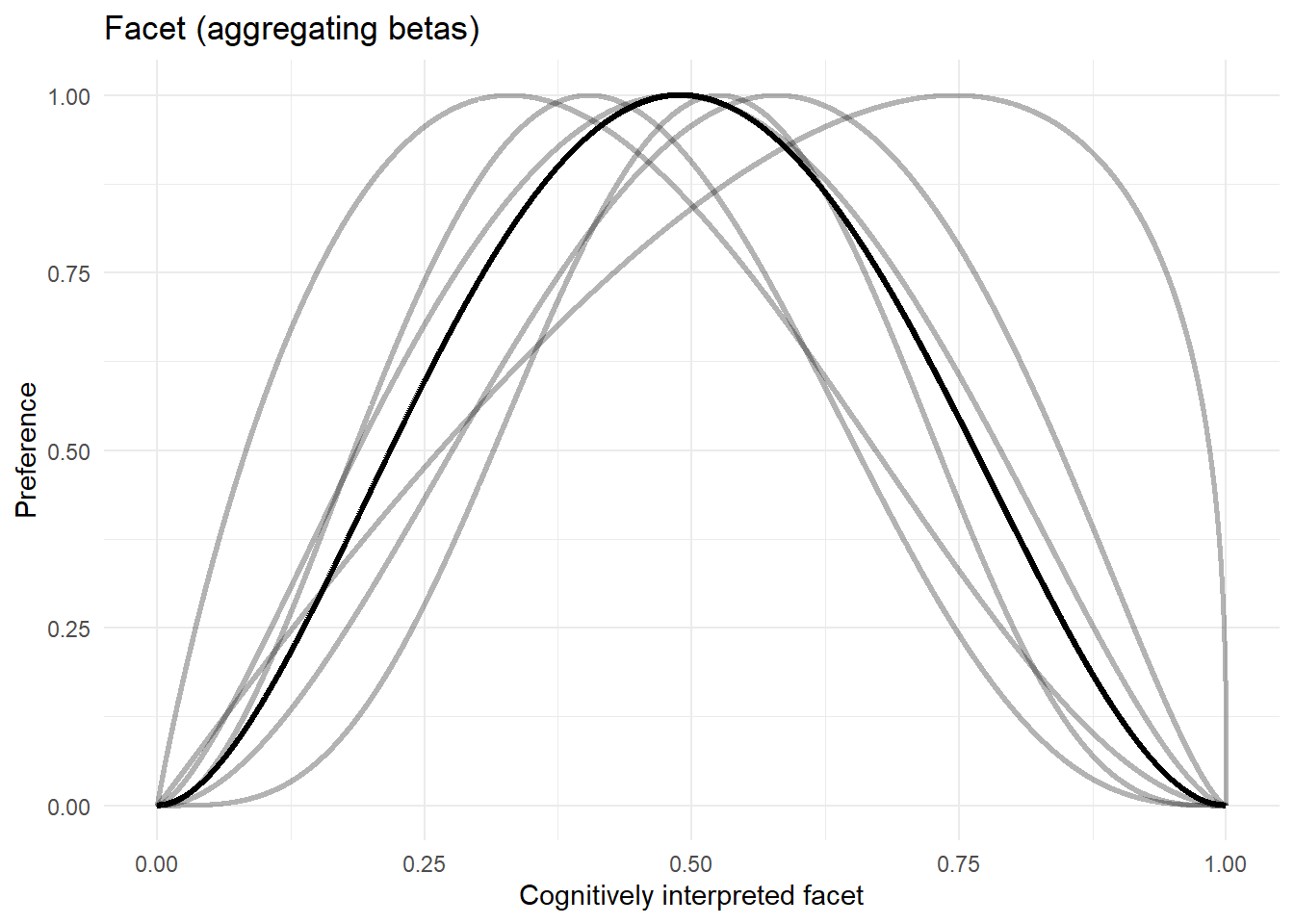
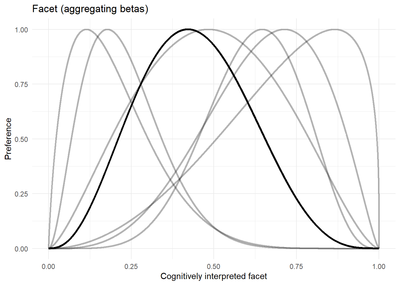
## Aggregating beta parameters
```{r, echo = FALSE}
plot_facet_beta <- function(tendencies, pvar, title, save = NULL) {
x <- seq(0, 1, 0.0001)
len <- length(tendencies * pvar)
df <- features_dist(
x = x,
tendencies = tendencies,
pvar = pvar
)
df$alpha <- 0.3
facet <- df %>%
group_by(x) %>%
summarise(
a = mean(a),
b = mean(b),
.groups = "drop"
)
facet$freq <- dbeta(facet$x, facet$a, facet$b)
facet$mode <- (facet$a - 1) / (facet$a + facet$b - 2)
facet$max <- ifelse(is.na(facet$mode), facet$freq, dbeta(facet$mode, facet$a, facet$b))
facet$probx <- facet$freq / facet$max
plt <- ggplot(
df, aes( x = x, y = probx, group = set)) +
geom_line(aes(alpha = alpha), linewidth = 1) +
scale_alpha_identity() +
geom_line(
data = facet,
aes(x = x, y = probx),
inherit.aes = FALSE,
linewidth = 1.2,
color = "black" ) +
labs(
x = "Cognitively interpreted facet",
y = "Preference",
title = title ) +
theme_minimal()
if (!is.null(save)) {
dir_path <- "img"
dir.create(dir_path, recursive = TRUE, showWarnings = FALSE)
file_path <- file.path(dir_path, paste0(save, ".png"))
ggsave(filename = file_path,
plot = plt,
width = 8,
height = 4,
units = "in",
dpi = 300)
}
plt
}
```
```{r}
plot_facet_beta(tendencies_1, pvar_1, "Facet (aggregating betas)")
plot_facet_beta(tendencies_2, pvar_2, "Facet (aggregating betas)", save = "Facet_beta")
```
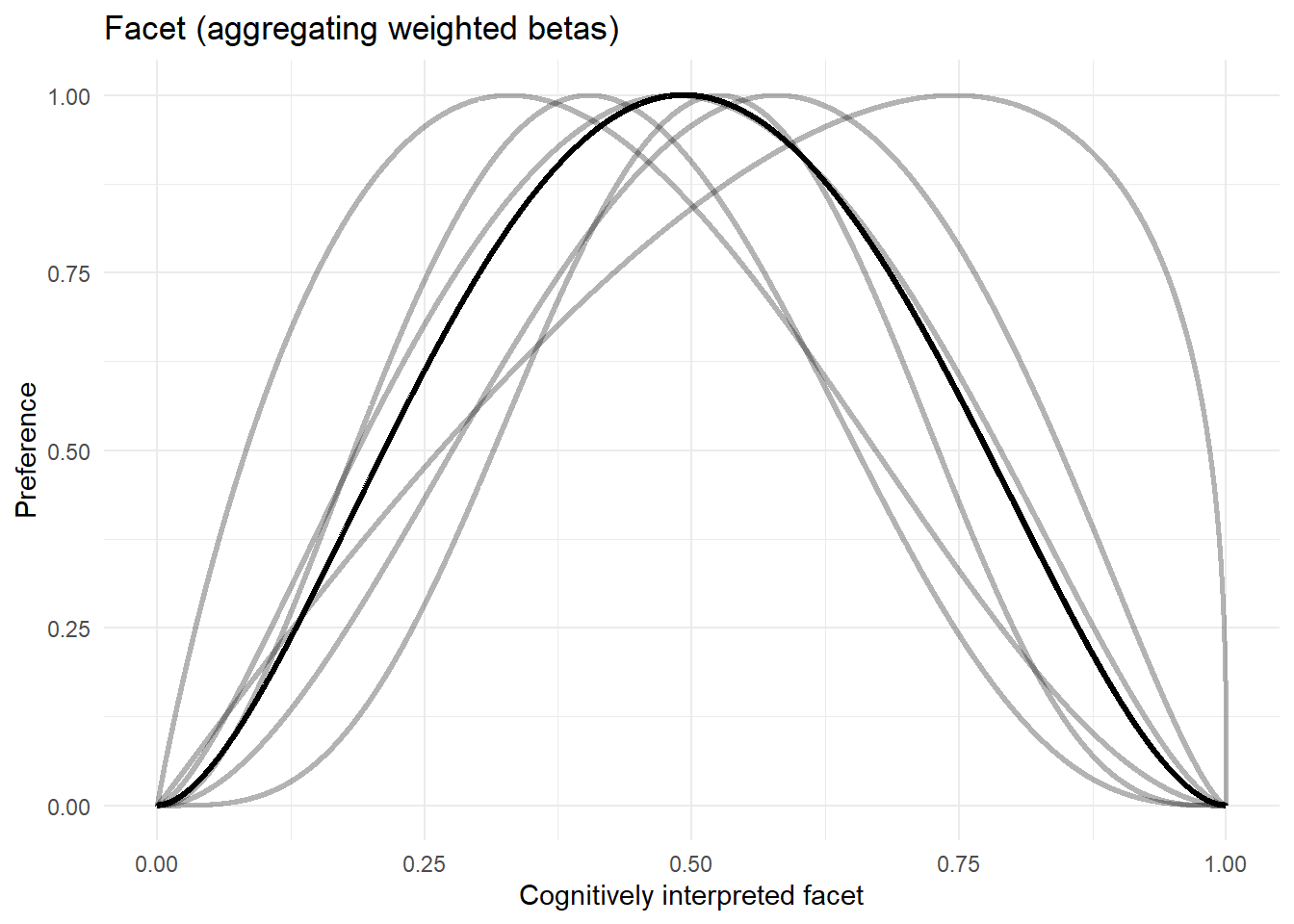
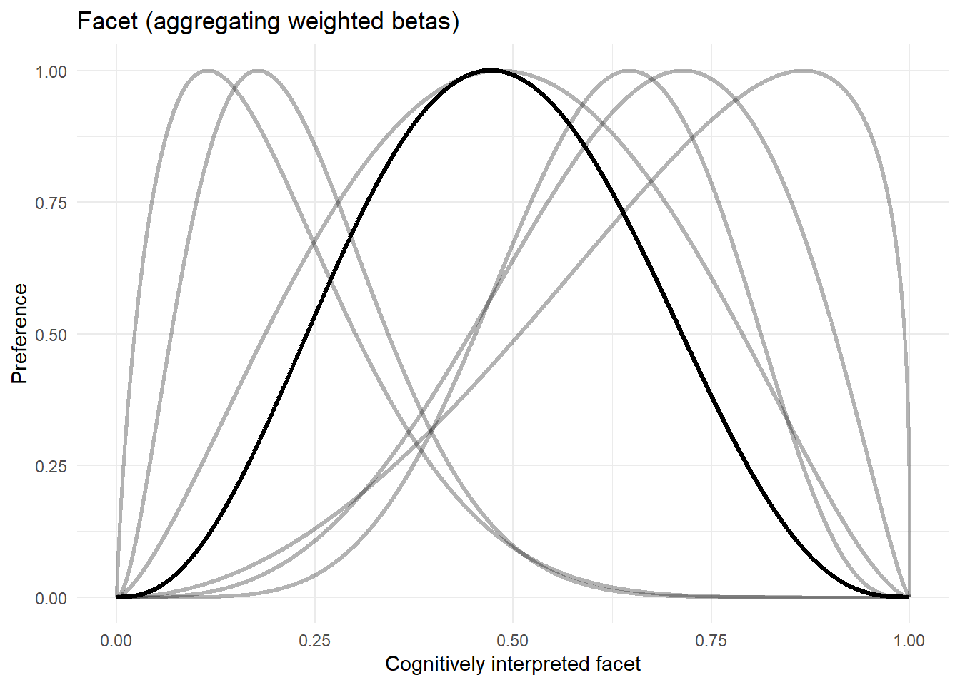
## Aggregating weighted beta parameters
```{r}
facets_1 <- df_1 %>%
    group_by(x) %>%
    summarise(
    a = weighted.mean(a, 1/max),
    b = weighted.mean(b, 1/max),
    .groups = "drop"
    )
```
```{r, echo = FALSE}
plot_facet_wbeta <- function(tendencies, pvar, title, save = NULL) {
x <- seq(0, 1, 0.0001)
len <- length(tendencies * pvar)
df <- features_dist(
x = x,
tendencies = tendencies,
pvar = pvar
)
df$alpha <- 0.3
facet <- df %>%
group_by(x) %>%
summarise(
a = weighted.mean(a, 1/max),
b = weighted.mean(b, 1/max),
.groups = "drop"
)
facet$freq <- dbeta(facet$x, facet$a, facet$b)
facet$mode <- (facet$a - 1) / (facet$a + facet$b - 2)
facet$max <- ifelse(is.na(facet$mode), facet$freq, dbeta(facet$mode, facet$a, facet$b))
facet$probx <- facet$freq / facet$max
plt <- ggplot(
df, aes( x = x, y = probx, group = set)) +
geom_line(aes(alpha = alpha), linewidth = 1) +
scale_alpha_identity() +
geom_line(
data = facet,
aes(x = x, y = probx),
inherit.aes = FALSE,
linewidth = 1.2,
color = "black" ) +
labs(
x = "Cognitively interpreted facet",
y = "Preference",
title = title ) +
theme_minimal()
if (!is.null(save)) {
dir_path <- "img"
dir.create(dir_path, recursive = TRUE, showWarnings = FALSE)
file_path <- file.path(dir_path, paste0(save, ".png"))
ggsave(filename = file_path,
plot = plt,
width = 8,
height = 4,
units = "in",
dpi = 300)
}
plt
}
```
```{r}
plot_facet_wbeta(tendencies_1, pvar_1, "Facet (aggregating weighted betas)")
plot_facet_wbeta(tendencies_2, pvar_2, "Facet (aggregating weighted betas)", save = "Facet_wbeta")
```
# \< [Back](../Personality.qmd#Facets)