These parameters are either determined by the situation (cog_res) or by the abilities of the agent (aff_cop). The parameter aff_cop is assumed to be stable, but it can be modified through interventions.
cog_res<-0.5# Weighting factor for the ideal self-conceptaff_cop<-0.5# Affective coping abilities
Self-Concepts
The self-concepts can either be defined a priori or dynamically updated throughout the simulation as a function of the accumulated experiences.
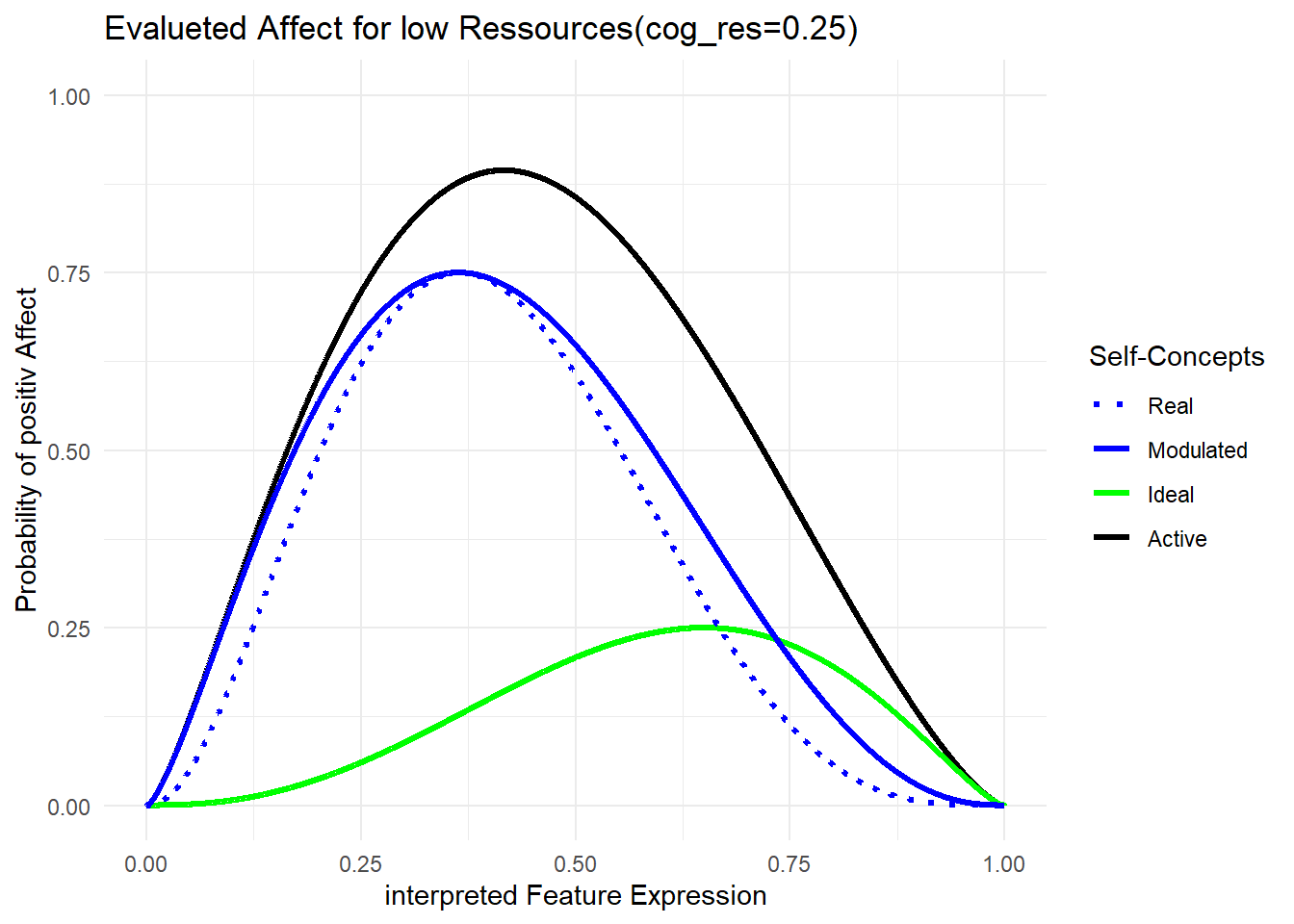
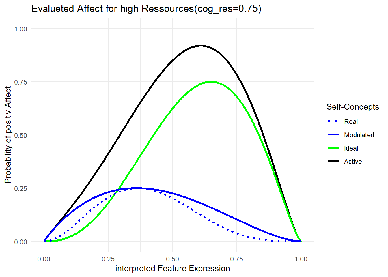
Ultimately, a weighting is applied to determine the affect that is active in a given situation. When cog_res = 1, affect is determined exclusively by the ideal self-concept. When cog_res = 0, affect is determined solely by the modulated real self-concept, as defined below by affective coping abilities.
by Affective Coping Abilities
It is assumed that, at maximal coping ability, the variance can be doubled. However, this increase is only realised if sufficient cognitive resources are available.
In addition, it must be ensured that pvar does not exceed 1, which corresponds to the maximum variance defined in the model. Furthermore, due to the skewness of beta distributions, the mean must be adjusted accordingly to ensure that the location of the maximum (mode) remains constant.
plot_aff_modeling(aff_cop, 0.25, real_sc_m, real_sc_v, ideal_sc_m, ideal_sc_v, title ="Evalueted Affect for low Ressources(cog_res=0.25)", save ="Affektive_Evaluation_low_Res")
plot_aff_modeling(aff_cop, 0.75, real_sc_m, real_sc_v, ideal_sc_m, ideal_sc_v, title ="Evalueted Affect for high Ressources(cog_res=0.75)", save ="Affektive_Evaluation_high_Res")